Andy Jones
Dirichlet process mixture models
\(\DeclareMathOperator*{\argmin}{arg\,min}\) \(\DeclareMathOperator*{\argmax}{arg\,max}\)
Mixture models provide a principled, Bayesian approach to clustering. However, finite mixture models require the number of components to be specified before fitting the model. In general, this is a difficult task and may require expensive techniques like cross-validation to select the number of components.
Infinite mixture models circumvent this problem by modeling the number of components directly. By incorporating this as part of the model, we can flexibly estimate the optimal number of components from the data, and even obtain a posterior over the number of components.
This post reviews one of the most popular infinite mixture models: the Dirichlet process mixture model (DPMM). First, we briefly review the Dirichlet distribution, and then we describe Dirichlet processes and DPMMs.
Dirichlet distribution
The Dirichlet distribution is a $K$-dimensional distribution over the $K-1$ simplex. A sample from a Dirichlet is a $K$-dimensional nonnegative vector that sums to one:
\[\mathbf{x} \sim \text{Dir}(\boldsymbol{\alpha}),~~~\sum\limits_{k=1}^K x_k = 1.\]The parameter vector $\boldsymbol{\alpha}$ controls the concentration of density around each index. Recall the form of the PDF for the Dirichlet distribution:
\[p(\mathbf{x} | \alpha_1, \dots, \alpha_K) = \frac{1}{B(\boldsymbol{\alpha})} \prod\limits_{k=1}^K x_k^{\alpha_k - 1}\]where $B(\cdot)$ is the beta function. The Dirichlet is a popular prior for categorical variables with $K$ categories. We can visualize the density of a $3$-dimensional Dirichlet below. In this animation, we plot the Dirichlet density (brighter colors indicate greater density) over the first two coordinates. (Note that $x_3$ is determined by $x_1, x_2$ due to the summation constraint.)
We can see that a higher value of $\alpha_k$ implies a higher concentration of density near index $k$.
Dirichlet-based clustering models
A common use of the Dirichlet distribution is in specifying a prior for the component assignments in a mixture model. For example, consider a Gaussian mixture model:
\[p(\mathbf{x} | \theta) = \sum\limits_{k=1}^K \pi_k \mathcal{N}(\mu_k, \Sigma_k)\]where $\mathbf{x} \in \mathbb{R}^p$ is a data point, $\theta$ are the cluster-specific parameters, and $\pi_k$ is the prior probability that $\mathbf{x}$ belongs to cluster $k$ with $\sum_k \pi_k = 1$.
A common choice for a prior distribution on $\boldsymbol{\pi}$ is a Dirichlet distribution,
\[\boldsymbol{\pi} \sim \text{Dir}(\underbrace{\alpha / K, \dots, \alpha / K}_{\text{$K$ times}}).\]The full generative model can then be written as follows:
\begin{align} \mathbf{x}_i | c_i, \theta &\sim \mathcal{N}(\boldsymbol{\mu}_{c_i}, \Sigma_{c_i}) \\ c_i | \boldsymbol{\pi} &\sim \text{Discrete}(\pi_1, \dots, \pi_K) \\ \boldsymbol{\pi} | \alpha &\sim \text{Dir}(\alpha / K, \dots, \alpha, K) \end{align}
where $c_i \in [K]$ is the cluster membership indicator for sample $i$. Note that we may additionally choose to place priors on the cluster-specific parameters $\{(\boldsymbol{\mu}_k, \Sigma_k)\}_{k=1}^K$.
In this type of finite mixture model, inference is typically carried out using expectation maximization (EM). EM is an iterative algorithm that alternates between finding the expectation of the $\log$ likelihood and maximizing the posterior with respect to the parameters $\theta$.
Dirichlet processes
A Dirichlet process is a stochastic process whose samples are probability distributions. In particular, given a “base” distribution $p_0$ and a nonnegative scalar $\alpha \in \mathbb{R}_+$, we denote a Dirichlet process as $DP(p_0, \alpha)$. A given Dirichlet process is defined on a particular set $S$ (e.g., this could be the real line). If a function is drawn from this process, $f \sim DP(p_0, \alpha)$, then the definition of a DP says that for any finite partition of $S$ given by $\{B_i\}_{i=1}^n$, it holds that
\[[f(B_1), \cdots, f(B_n)] \sim \text{Dir}(\alpha p_0(B_1), \cdots, \alpha p_0(B_n)).\]As we’ll see below, Dirichlet processes are useful for generalizing the above mixture model.
Dirichlet process mixture models
A Dirichlet process mixture model arises as a limiting case of the above finite mixture model as we let $K \to \infty$. To see this, let’s first find the distribution of the indicator variables $\mathbf{c}$ for the finite mixture model. Let $n_k$ denote the number of samples belonging in component $k$. Then we have
\begin{align} p(\mathbf{c}, \boldsymbol{\pi} | \alpha) &= p(\mathbf{c} | \boldsymbol{\pi}) p(\boldsymbol{\pi} | \alpha) \\ &= \prod\limits_{k=1}^K \pi_k^{n_k} \cdot \text{Dir}(\boldsymbol{\pi} | \alpha/K, \dots, \alpha/K) \\ &= \prod\limits_{k=1}^K \pi_k^{n_k} \cdot \frac{1}{B(\alpha/K)} \prod\limits_{k=1}^K \pi_k^{\alpha/K - 1} \\ &= \frac{\Gamma(\alpha)}{\Gamma(\alpha/K)^K} \prod\limits_{k=1}^K \pi_k^{n_k + \alpha/K - 1}. \end{align}
Integrating out the mixing proportions $\boldsymbol{\pi}$, we have
\begin{align} p(\mathbf{c} | \alpha) &= \int p(\mathbf{c}, \boldsymbol{\pi} | \alpha) d\boldsymbol{\pi} \\ &= \frac{\Gamma(\alpha)}{\Gamma(\alpha/K)^K} \int \prod\limits_{k=1}^K \pi_k^{n_k + \alpha/K - 1} d\boldsymbol{\pi} \\ &= \frac{\Gamma(\alpha)}{\Gamma(n + \alpha)} \prod\limits_{k=1}^K \frac{\Gamma(n_k + \alpha/K)}{\Gamma(\alpha/K)}. \end{align}
From this expression, we can then get the prior probability that the indicator for a specific point belongs to a particular component. Without loss of generality, assume we’d like the prior that the $n$th data point belongs to cluster $k$. Then, writing out this conditional prior, we have:
\begin{align} p(c_n = k | c_1, \dots, c_{n-1}, \alpha) &= \frac{p(c_n = k, c_1, \dots, c_{n-1}, \alpha)}{p(c_1, \dots, c_{n-1}, \alpha)} \\ &= \frac{\frac{\Gamma(\alpha)}{\Gamma(n + \alpha)} \prod\limits_{k^\prime=1}^K \frac{\Gamma(n_{-n, k^\prime} + 1_{(k^\prime = k)} + \alpha/K)}{\Gamma(\alpha/K)}}{\frac{\Gamma(\alpha)}{\Gamma(n - 1 + \alpha)} \prod\limits_{k^\prime=1}^K \frac{\Gamma(n_{-n, k^\prime} + \alpha/K)}{\Gamma(\alpha/K)}} \end{align}
where $1_{(k^\prime = k)}$ is the indicator function (which is $1$ when $k^\prime = k$ and $0$ otherwise). We can now cancel and rearrange terms:
\begin{align} p(c_n = k | c_1, \dots, c_{n-1}, \alpha) &= \frac{\frac{1}{\Gamma(n + \alpha)} \prod\limits_{k^\prime=1}^K \Gamma(n_{-n, k^\prime} + 1_{(k^\prime = k)} + \alpha/K)}{\frac{1}{\Gamma(n - 1 + \alpha)} \prod\limits_{k^\prime=1}^K \Gamma(n_{-n, k^\prime} + \alpha/K)} \\ &= \frac{\Gamma(n - 1 + \alpha)}{\Gamma(n + \alpha)} \cdot \frac{\Gamma(n_{-n, k^\prime} + 1 + \alpha/K)}{\Gamma(n_{-n, k^\prime} + \alpha/K)}. \end{align}
Recalling that, for any $x$, $x \Gamma(x) = \Gamma(x + 1)$, we can simplify this expression as follows:
\begin{align} &\frac{\Gamma(n - 1 + \alpha)}{\Gamma(n + \alpha)} \cdot \frac{\Gamma(n_{-n, k^\prime} + 1 + \alpha/K)}{\Gamma(n_{-n, k^\prime} + \alpha/K)} \\ =& \frac{\Gamma(n - 1 + \alpha)}{(n - 1 + \alpha) \Gamma(n - 1 + \alpha)} \cdot \frac{(n_{-n, k^\prime} + \alpha/K) \Gamma(n_{-n, k^\prime} + \alpha/K)}{\Gamma(n_{-n, k^\prime} + \alpha/K)} \\ =& \frac{n_{-n, k^\prime} + \alpha/K}{n - 1 + \alpha}. \end{align}
Now we can take the limit as $K \to \infty$. Note that we’re discussing a finite set of data points, while the number of components is going to infinity. Thus, there will be components without any data points, and we must treat components with and without existing data points separately. For components with data points already assigned to them, we can easily see that the term $\alpha/K$ will go to zero, so we have
\[p(c_i = k | c_{-i}, \alpha) = \frac{n_{-i, k}}{n - 1 + \alpha}.\]Then we must find the prior for all other components that are empty. Assume that there are $K$ components that already contain data points. Since the prior must sum to one, we have
\begin{align} &\sum_{k=1}^K p(c_i = k | c_{-i}, \alpha) + p(c_i = c_{i^\prime} \text{ for all } i \neq i^\prime | c_{-i}, \alpha) = 1 \\ \implies& p(c_i = c_{i^\prime} \text{ for all } i \neq i^\prime | c_{-i}, \alpha) = 1 - \frac{\sum_{k=1}^K n_{-i, k}}{n - 1 + \alpha} \\ \implies& p(c_i = c_{i^\prime} \text{ for all } i \neq i^\prime | c_{-i}, \alpha) = \frac{n - 1 + \alpha}{n - 1 + \alpha} - \frac{n - 1}{n - 1 + \alpha} \\ \implies& p(c_i = c_{i^\prime} \text{ for all } i \neq i^\prime | c_{-i}, \alpha) = \frac{\alpha}{n - 1 + \alpha}. \end{align}
Notice that the prior for a particular component grows as its number of constituent data points increases. For components without any points assigned to them, we place a prior on each of these that is effectively equivalent to allocating “pseudo-samples” of size $\alpha$ to each of them.
We can equivalently write this model in terms of a Dirichlet process. Specifically, we can place a DP prior on the cluster-specific parameters $\theta$. Let’s again assume that each component follows a Gaussian distribution, so our parameters are the mean and covariance of each sample, $\theta = \{\boldsymbol{\mu}_i, \Sigma_i\}_{i = 1}^n$.
\begin{align} \mathbf{x}_i &\sim \mathcal{N}(\boldsymbol{\mu}_i, \Sigma_i) \\ (\boldsymbol{\mu}_i, \Sigma_i) &\sim f \\ f &\sim DP(p_0, \alpha). \end{align}
In words, the generative process works as follows:
- Draw a distribution $f$ from a DP that is a discrete distribution over model parameters.
- Draw the mean and covariance for sample $i$ from $f$.
- Draw sample $i$ from a multivariate Gaussian with these parameters.
Inference
The most popular approach for fitting DPMMs is to use some form of Markov chain Monte Carlo (MCMC). Many sophisticated sampling approaches have been developed for infinite mixture models, but we’ll examine one simple approach in this post, as shown in the example below.
Example
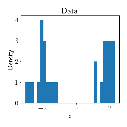
For illustration, let’s consider a simple example. Suppose we observe one-dimensional data that we’d like to cluster. We draw a synthetic dataset from the following mixture of two Gaussians:
\[x_i \sim 0.5 \mathcal{N}(-2, 1) + 0.5 \mathcal{N}(2, 1).\]Below is a histogram of our data.
Now, let’s perform inference using a DPMM. Suppose we don’t know the true number of clusters in the data, and we also don’t know the mean of each cluster. Our model of the data is then
\begin{align} \mathbf{x}_i &\sim \mathcal{N}(\mu_i, \sigma^2_0) \\ \mu_i &\sim f \\ f &\sim DP(p_0, \alpha) \\ p_0 &= \mathcal{N}(0, 1) \end{align}
where we assume $\sigma^2_0$ is known for simplicity. In other words, we have a Dirichlet mixture of Gaussians. The primary quantities of interest for us are going to be the number of unique mixture components and the associated mean $\mu$ of each of those components.
To perform inference in this model, we’ll take a sampling-based approach from a 2000 paper by Radford Neal. To start, at any given iteration of the sampler, we will have a vector of parameters, each of which corresponds to a data point. Given $n$ data points, denote our parameter vector as
\[\boldsymbol{\mu} = [\mu_1, \mu_2, \cdots, \mu_n]^\top.\]Some of these parameters will be repeats of each other, indicating that these samples belong to the same cluster. In a DPMM sampler, we’d like to sample new parameters from the distribution of existing parameters with probability proportional to the count of each unique existing parameter. This is the “rich get richer” property of Dirichlet processes: components with larger numbers of samples will tend to receive new samples more often than smaller components.
In particular, we can form a discrete distribution over the existing parameters and sample from this distribution. We’ll assign a weight to each parameter based on the data likelihood under each parameter. When we draw a new sample for data point $x_i$, we can represent this density as
\[\sum\limits_{j\neq i} \mathcal{N}(x_i | \mu_j, 1) \delta(\mu_j)\]where we use the notation $\mathcal{N}(x_i | \mu_j, 1)$ to denote the likelihood PDF evaluation at $x_i$, and $\delta(\mu_j)$ is a point mass at $\mu_j$.
Now we have a way to sample existing parameters, but we’d also like to have the opportunity to sample parameter values that are not currently in our parameter vector. We can think of this as an “exploration vs. exploitation” tradeoff: we want to cluster the data based on the parameter values that we already have, but we also want to randomly explore new parts of the parameter space with some probability.
To do so, we’ll tweak our above density slightly. Now, with probability proportional to $\alpha p(x_i)$ (where $p(x_i$ is the marginal likelihood of $x_i$), we’ll sample from the posterior. The density from which we’ll sample is now
\[\mu_i | \boldsymbol{\mu}_{-i}, x_i \sim \frac1Z \left[\underbrace{\sum\limits_{j\neq i} \mathcal{N}(x_i | \mu_j, 1) \delta(\mu_j)}_{\text{Existing sample}} + \underbrace{\alpha p(x_i) p(\mu_i | x_i)}_{\text{New sample}}\right].\]where $Z$ is a normalizing constant, and $\boldsymbol{\mu}_{-i}$ is the parameter vector without sample $i$. Because our model is fully Gaussian, we can compute $p(x_i)$ and $p(\mu_i | x_i)$ in closed form (however, this won’t be true in general).
Putting this all together, we have the following algorithm:
- For $\text{iter} = 1, \dots, \text{# iters}$:
- For $i = 1, \dots, n$:
- Sample $\widehat{\mu}_i$ from $p(\mu_i | \boldsymbol{\mu}_{-i}, x_i).$
- Save $\widehat{\mu}_i$ in the history of samples.
- Update the $i$th element of the parameter vector $\boldsymbol{\mu}$ with $\widehat{\mu}_i$.
- For $i = 1, \dots, n$:
Let’s run this on our data and see how it turns out. In the plot below, we show the samples drawn from the algorithm above for our model. The x axis shows the iteration number of the sampler, and the y axis indicates the sample value. The width of the blobs across time is proportional to the number of samples assigned to the component with that parameter value.
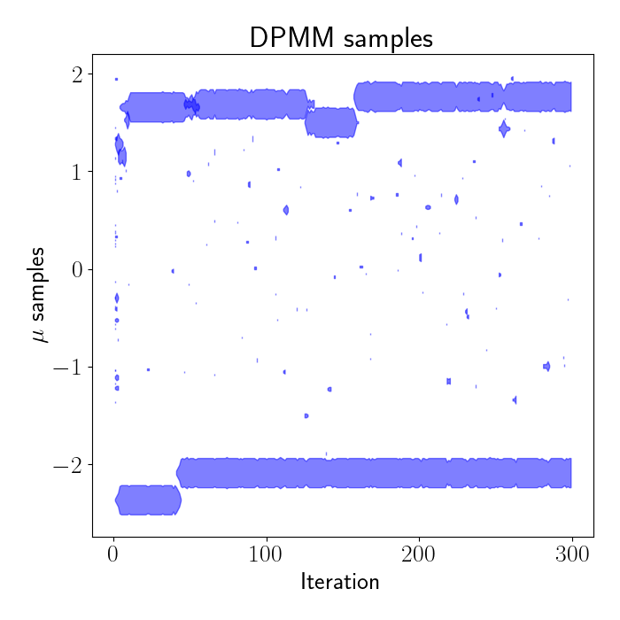
We can see that the samples quickly split into two clusters: one near $\mu=2$ and another near $\mu=-2$, which are exactly the true cluster means of our data. The speckles on the left side of the plot at iteration $0$ show that we initialize our parameters randomly, but they quickly begin clustering together due to the clustering properties of Dirichlet processes. In practice, we throw out these early samples and treat the initial iterations as “burn-in” iterations.
We can also view the evolution of the samples in terms of the actual distributions modeling the data. In the animation below, the red curves indicate the mixture component distributions over the first 30 iterations of sampling. The blue density is the histogram of data.
We can see that the components quickly end up being two Gaussians centered on the two data clusters.
After the sampler is done running (here, for several hundred iterations), we can look at the final estimate of the posterior. Below, the left plot shows the posterior for $\mu$, and the right plot shows the posterior over the number of components.
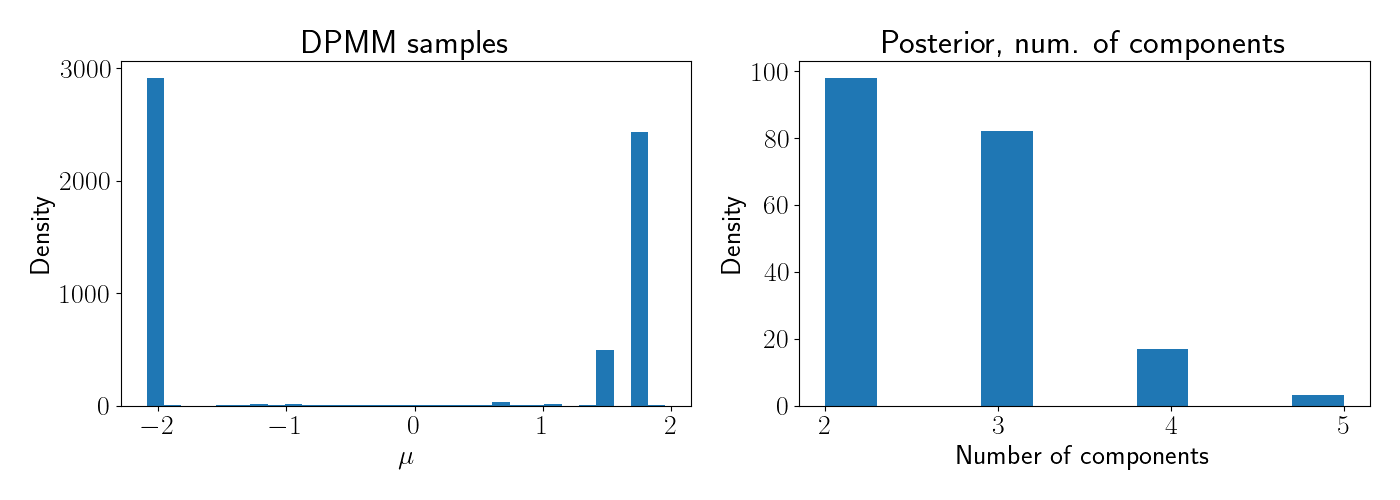
Clearly the modal value for the number of components is at $2$, as expected.
Conclusion
Dirichlet process mixture models provide an attractive alternative to finite mixture models because they don’t require the modeler to specify the number of components a priori.
Code
Code for running the examples above can be found in the GitHub repo associated with this post.
References
- Neal, Radford M. “Markov chain sampling methods for Dirichlet process mixture models.” Journal of computational and graphical statistics 9.2 (2000): 249-265.
- Yee Whye Teh’s notes on the Dirichlet process.