Andy Jones
The ubiquity of degrees of freedom
\(\DeclareMathOperator*{\argmin}{arg\,min}\) \(\DeclareMathOperator*{\argmax}{arg\,max}\)
The concept of “degrees of freedom” plays an important role in many areas of statistics, engineering, and mathematics. Here, we explore several contexts in which degrees of freedom are relevant along with some useful visualizations.
Generic definition
Generically, the degrees of freedom of a random vector is the number of elements of that vector that can vary independently of one another. Another interpretation of this definition is that the degrees of freedom of a random vector is the intrinsic dimensionality of the space in which the vector resides.
To give a more specific example, consider a random vector,
\[\mathbf{x} = \begin{bmatrix} x_1 \\ x_2 \end{bmatrix}.\]Without any further constraints, $\mathbf{x}$ has two degrees of freedom because $x_1$ and $x_2$ can both vary independently of one another. Equivalently, $\mathbf{x}$ lives in a two-dimensional space.
Now, suppose we add a constraint that must be satisfied:
\[x_2 = 3 x_1.\]In this case, as soon as we choose $x_1$, we no longer have freedom to choose any value for $x_2$. We must choose three times the value we chose for $x_1$. If we choose $x_1=3$, then we are immediately required to choose $x_2=9$. Similarly, choosing $x_2$ strips us of our freedom to choose $x_1$. Thus, with this additional constraint, $\mathbf{x}$ has just one degree of freedom.
Systems of linear equations
We can generalize our understanding of degrees of freedom from the previous section, where we saw that when we applied a linear constraint to the vector, we lost a degree of freedom. Consider a linear system of equations in matrix form:
\[\mathbf{A}\mathbf{x} = \mathbf{y},\]where $\mathbf{x} \in \mathbb{R}^m$ is our random vector, $\mathbf{A}$ is an $n \times m$ matrix, and $\mathbf{y}$ is an $n$-vector. If we were to write out each row of the linear system, we can see each individual equation:
\begin{align} a_{11} x_1 + a_{12} x_1 + \cdots + a_{1m} x_m &= y_1 \\ a_{21} x_1 + a_{22} x_1 + \cdots + a_{2m} x_m &= y_2 \\ \vdots & \\ a_{n1} x_1 + a_{n2} x_1 + \cdots + a_{nm} x_m &= y_n. \end{align}
Our example from the previous section was an instance of this more general system where $n=1, m=2.$
In general systems of linear equations like this, there are $m - n$ degrees of freedom. If $n=m$, then there are zero degrees of freedom and all of the elements of $\mathbf{x}$ are fully constrained once $\mathbf{A}$ is known. If $n < m$, then we have extra degrees of freedom, and the system has more variables than constraints, implying that there will be multiple solutions to the system of equations. If $n > m$, then there are negative degrees of freedom since there are more constraints than variables.
Linear regression
Recall the standard linear regression problem with predictors $\mathbf{X} \in \mathbb{R}^{n \times p},$ response $\mathbf{y} \in \mathbb{R}^n,$ coefficient vector $\boldsymbol{\beta} \in \mathbb{R}^p,$ and noise vector $\boldsymbol{\epsilon} \in \mathbb{R}^n:$
\[\mathbf{y} = \mathbf{X}\boldsymbol{\beta} + \boldsymbol{\epsilon}\]By solving $\min_{\boldsymbol{\beta}} ||\mathbf{y} - \mathbf{X}\boldsymbol{\beta}||^2,$ we obtain the OLS estimator:
\[\widehat{\boldsymbol{\beta}} = (\mathbf{X}^\top \mathbf{X})^{-1} \mathbf{X}^\top \mathbf{y}.\]Fitted values are then given by
\[\mathbf{X} \widehat{\boldsymbol{\beta}} = \underbrace{\mathbf{X} (\mathbf{X}^\top \mathbf{X})^{-1} \mathbf{X}^\top}_{\mathbf{H}} \mathbf{y},\]where $\mathbf{H}$ is a projection matrix that is often called the “hat matrix”. The hat matrix also gives a route to calculating the number of degrees of freedom. Specifically, the number of degrees of freedom is given by the trace of the hat matrix (equivalently, the sum of the eigenvalues of the hat matrix):
\[\text{tr}(\mathbf{H}).\]Note that $\mathbf{H}$ is a projection matrix in the sense that it projects the response vector $\mathbf{y}$ onto the column space of $\mathbf{X}.$ This implies that if $\mathbf{X}$ is full rank, then the degrees of freedom will be $\min(n, p).$ In most regression settings, we assume that $n > p,$ implying that there are usually $p$ degrees of freedom. When $n > p,$ or when the columns of $\mathbf{X}$ are linearly dependent, then there will be fewer than $p$ degrees of freedom.
Ridge regression
When a linear regression model is underconstrained, a common solution is to reduce the model’s variance by regulairizing it. Ridge regression is one popular regularized linear model. Recall the ridge regression optimization problem:
\[\min_{\boldsymbol{\beta}} \|\mathbf{y} - \mathbf{X}\boldsymbol{\beta}\|^2 + \lambda \|\boldsymbol{\beta}\|^2,\]where $\lambda > 0$ controls the strength of the regularization. The ridge estimator is
\[\widehat{\boldsymbol{\beta}} = (\mathbf{X}^\top \mathbf{X} + \lambda \mathbf{I})^{-1} \mathbf{X}^\top \mathbf{y}.\]We can interpret regularization through the lens of degrees of freedom as well. Specifically, we can see that increasing the amount of regularization in a model decreases its degrees of freedom. To see this, first note that, for the ridge estimator, the hat matrix $\mathbf{H}$ is given by
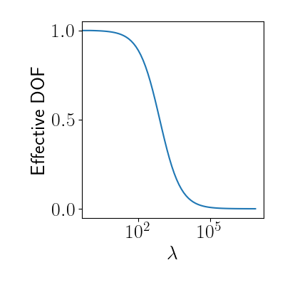
\[\mathbf{H} = \mathbf{X} (\mathbf{X}^\top \mathbf{X} + \lambda \mathbf{I})^{-1} \mathbf{X}^\top.\]We then say that the effective degrees of freedom is given by $\text{tr}(\mathbf{H}).$ Note that the effective degrees of freedom will decline as $\lambda$ increases. In the limit where $\lambda \to \infty$, the effective degrees of freedom goes to zero. This intuitively makes sense in the ridge regression context: as $\lambda\to\infty,$ all model coefficients go to zero, leaving us with no freedom to choose them.
Sample mean and standard deviation
Degrees of freedom also appear in more basic statistical estimators, like the sample mean and variance. Suppose we have two samples, $x_1$ and $x_2$ drawn from the same population that has true mean $\mu$ and true variance $\sigma^2.$ Their sample mean is given by
\begin{equation} \widehat{\mu} = \frac12(x_1 + x_2). \tag{1} \label{eq:sample_mean} \end{equation}
The sample mean is easily shown to be unbiased:
\[\mathbb{E}[\widehat{\mu}] = \frac12 \left(\mathbb{E}[x_1] + \mathbb{E}[x_2]\right) = \frac12 (2 \mu) = \mu.\]Recall the sample estimator for the variance:
\[\widehat{\sigma^2} = \frac12 (x_1 - \mu)^2 + \frac12 (x_2 - \mu)^2.\]When $\mu$ is known, $\widehat{\sigma^2}$ is an unbiased estimator for $\sigma^2$:
\begin{align} \mathbb{E}[\widehat{\sigma^2}] &= \mathbb{E}[\frac12 (x_1^2 - 2 x_1 \mu + \mu^2 + x_2^2 - 2 x_2 \mu + \mu^2)^2] \\ &= \frac12\mathbb{E}[x_1^2] + \frac12\mathbb{E}[x_2^2] - \mu \mathbb{E}[x_1] - \mu \mathbb{E}[x_2] + 2 \mu^2 \\ &= \sigma^2 - 2 \mu^2 + 2 \mu^2 \\ &= \sigma^2. \end{align}
However, if $\mu$ is unknown and we must use the sample estimator $\widehat{\mu}$, the variance estimator is no longer unbiased. Let’s show this.
Rearranging Equation \ref{eq:sample_mean}, we know that $x_1 = 2 \widehat{\mu} - x_2.$ Plugging this into the equation for $\widehat{\sigma^2},$ we have
\begin{align} \widehat{\sigma^2} &= \frac12 (2 \widehat{\mu} - x_2 - \widehat{\mu})^2 + \frac12 (x_2 - \widehat{\mu})^2 \\ &= \frac12 (\widehat{\mu} - x_2)^2 + \frac12 (x_2 - \widehat{\mu})^2 \\ &= (x_2 - \widehat{\mu})^2. \end{align}
This estimator is now biased:
\begin{align} \mathbb{E}[\widehat{\sigma^2}] &= \mathbb{E}[(x_2 - \widehat{\mu})^2] \\ &= \mathbb{E}[(x_2 - \frac12 x_1 - \frac12 x_2)^2] \\ &= \mathbb{E}[(\frac12 x_2 - \frac12 x_1)^2] \\ &= \frac14 \left\{\mathbb{E}[x_2^2] - \mathbb{E}[2 x_1 x_2] + \mathbb{E}[x_1^2]\right\} \\ &= \frac14 \left\{\sigma^2 - 0 + \sigma^2 \right\} \\ &= \frac12 \sigma^2 \\ &\neq \sigma^2. \end{align}
Another way to interpret the biased and unbiased estimators for the sample variance is in terms of degrees of freedom. When we compute the sample mean $\widehat{\mu} = \frac12(x_1 + x_2),$ we are effectively incorporating a linear constraint for any future calculations we make. This is because, for any other statistics we compute, the values for $x_1$ and $x_2$ must satisfy the equation for the sample mean once $\widehat{\mu}$ is calculated. Thus, we have lost a degree of freedom.
When we then compute the sample variance, in practice we’re no longer using both samples to estimate it. This is because we already have our constraint from estimating the mean, so we effectively have a sample size of $1$ after that. However, if we still divide the sample variance calculation by $2$ (or the sample size $n$ in the more general case), we’re not accounting for our “effective” sample size correctly. Dividing by $1$ (or $n - 1$ in the general case) solves this issue.
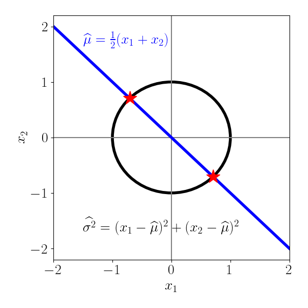
We can visualize this below, where we plot the allowable values for $x_1$ and $x_2$. After we calculate the sample mean, the linear constraint forces our choice of $x_1$ and $x_2$ to lie on the blue line. In other words, we’re selecting along one dimension. The circle represents the sample variance equation when the sample mean is $\widehat{\mu} = 0.$
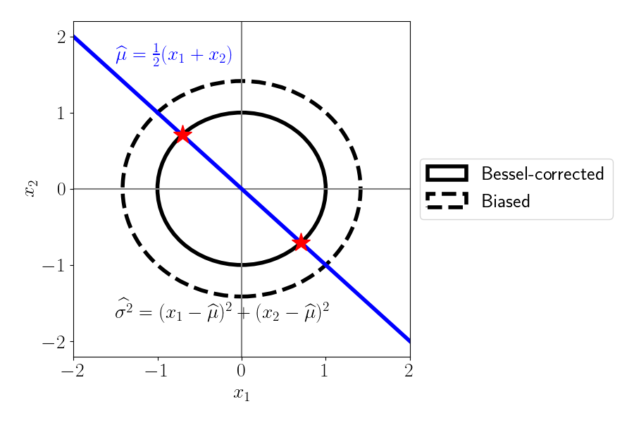
We can now show what happens if we don’t correct for the sacrificed degree of freedom. The solid black circle shows the same plot as above, with the bias-corrected sample variance calculation (often called the “Bessel-corrected” calculation). On the other hand, the dashed line shows the biased version, where we have divided by the original sample size, $2.$ We can see that if we don’t correct for the lost degree of freedom, the values of $x_1$ and $x_2$ are allowed to be larger (demonstrated by the fact that the dashed circle is larger). In other words, for a given sample, the variance will be estimated to be smaller than it actually is.
References
- Janson, Lucas, William Fithian, and Trevor J. Hastie. “Effective degrees of freedom: a flawed metaphor.” Biometrika 102.2 (2015): 479-485.