Andy Jones
COVID-19 Zoomposium notes
On 4/2/20, The Dana-Farber Cancer Institute and the Brown Institute at Columbia hosted a “zoomposium” (symposium via Zoom) about epidemiological modeling of the COVID-19 pandemic. These are my notes from the speakers’ presentations.
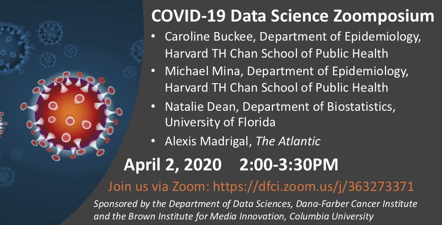
Flyer for the zoomposium:

I was only able to attend Profs. Buckee and Mina’s talks, but I hope to finish out the notes for the other talks once the recorded version is posted online.
Caroline Buckee
Professor Buckee focused her talk on explaining some of the mathematical and statistical models that are commonly used to model infectious diseases. She stressed that the goals of these models – as well as the actual models used – must change over the course of an outbreak. Specifically, if we divide an outbreak into an “early” stage and a “later” stage, common goals in these stages are:
- Early stage: Estimate basic parameters of the disease and the outbreak dynamics. These include the basic reproduction number, incubation period, latent period, duration of infection, etc.
- Later stage: Use models to evaluate the effectiveness of various interventions, and how to safely manage the end of the outbreak, as well as possible resurgences of the disease.
Early stage
One of the most fundamental measures of the infectiousness of a disease is called the basic reproduction number, denoted $R_0$. Indeed, the $R_0$ quickly became a well-known quantity early on in the coronavirus outbreak, as its estimates were widely reported on the news.
So what is the $R_0$? In words, it’s essentially the average number of people who will be infected by one person with the disease. Initial estimates of the $R_0$ for the coronavirus are around 2-3, which ranks it as solidly higher than H1N1 and Ebola.
Early on in an outbreak, the $R_0$ can be estimated statistically by fitting a growth rate curve to the cumulative number of cases. However, this is difficult because you have to make assumptions about the time to infection after exposure, and there are wide variations in testing practices (who gets tested, where they get tested, etc.).
As the outbreak progresses, it becomes more useful to estimate disease parameters mechanistically, rather than statistically. Mechanistic models can describe more precisely how transmission occurs, and it helps us to understand the disease dynamics more clearly.
In order to understand the basis of $R_0$ more thoroughly, we need to investigate a common mechanistic epidemiological model called the SIR model and its extension, the SEIR model.
SIR model
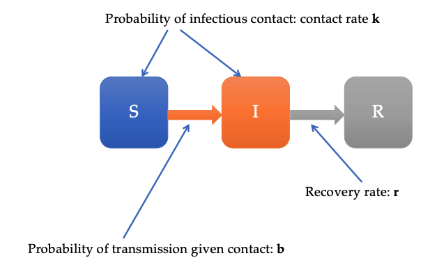
The SIR model – known as a “compartmental model” in epidemiology – bins each person in a population into one of three discrete states: susceptible (S), infectious (I), or recovered (R). Disease dynamics are described by the rate at which people transition between these states (usually modeled by a series of differential equations). This diagram from Prof. Buckee’s talk gives a graphical depiction of the model:

Note that we have the following probabilities:
\[b = \mathbb{P}[\text{transmission} \; | \; \text{contact}]\] \[k = \text{contact rate}\] \[r = \text{recovery rate}\]This implies that the rate at which people transition from $S$ to $I$ is $b k$.
If we also account for the rate at which people recover from the disease, we have that the overall rate of increase in infectious people is
\[R_0 = \frac{b k}{r}.\]This is the true underlying definition of $R_0$. Notice that there are three ways for the $R_0$ to increase:
- Higher $b$: higher probability of being infected if in contact with infectious person.
- Higher $k$: more contact with people.
- Lower $r$: slower recovery rate from the disease.
Importantly, initially people can really only control one of these: $k$, the rate of contact with other people. Intervention measures like social distancing are intended to reduce $k$, the rate of contact with other people, thereby reducing $R_0$.
The $R_0$ value is also highly context-specific: it varies depending on how different populations move around and interact with each other.
SEIR model
In many diseases, the transition from susceptible to infectious is not immediate. Rather, there’s an “incubation period” during which people have been exposed and infected, but aren’t infectious, so they can’t spread it to other people.
To account for this, an extra compartment can be added to the SIR model to form the SEIR model, where E stands for exposed. This extra compartment also changes $R_0$ estimates, as we now have to account for the transition rates into and out of the exposed state (see the Wikipedia entry for more details.
Here’s a graphical depiction of the SEIR model from Prof. Buckee’s talk (with slightly modified names for the transition rate parameters):

Another potential tweak to the SIR model is to separate the infectious state into two compartments: one for symptomatic people, and another for asymptomatic people. This could be especially important in the case of the coronavirus, since several results indicate that a nonnegligible fraction of infectious people might be asymptomatic (Liu et al, 2020). (We’ll be able to get a better estimate of this fraction as we move to antibody testing – more on that later.)
Evaluating interventions
As these initial models are being tweaked in the early stages of an outbreak, they can be used to start to assess the effectiveness of possible interventions. Mechanistic models allow us to ask questions of the form, ‘What happens with implementing X policy?’ (for example, mandatory school closures). We can then plan for various scenarios by running the models with a range of parameter settings, which will yield a range of possible outcomes.
Later stages
As an outbreak progresses and hopefully trends downward, it’s then important to think about the endgame. At this point, scientists should consider things like how long it will take for the disease to completely disappear, and whether a seasonal recurrence of the disease is possible.
Other useful points
- Notice that none of the above mentions forecasting. While there have been lots of forecasts floating around on the media and elsewhere, forecasting is difficult for pandemics because of the heterogenity in testing, and because the coronavirus is fairly unstudied.
- Often when projected scenarios are reported, a range of possible outcomes are reported. It’s common to mistakenly think that this range is deduced from multiple models that disagree with one another. In reality, these ranges often come from a single model in which particular parameter values are varied.
Michael Mina
Professor Mina focused his talk on the logistics of testing for the coronavirus.
Early missteps by the CDC
The initial fumbling of coronavirus testing in the United States is primarily attributable to early policies of the CDC that don’t make much sense in retrospect.
The first major policy was that all testing must be done by the CDC. On one hand, this policy makes sense to maintain the quality and authority of testing. On the other hand, this creates a clear bottleneck in the number and types of tests that can be created and administered. This disincentivized, or even prohibited, independent labs and large companies from creating new tests.
The second major policy was that the CDC would plan to create its own test, rather than use the one that had already been developed by the WHO. It took time for the CDC to create its own test, and it didn’t happen without a couple initial failures. At the same time, it was fairly clear that the WHO test was reliable, so there was no clear reason to opt for creating a new one.
On top of all of this, there was poor communication by the CDC about the status of testing, as well as whether other labs were allowed to use their resources for testing. This handling of the situation would have been okay for a disease like Ebola, which has low transmission rates. However, the coronavirus situation escalated rapidly, and the CDC’s action ultimately stifled the introduction of new tests.
Current testing policy
The FDA and CDC have now started to significantly deregulate the testing process. Typically, if a lab wants to develop a new test for a disease, the lab has to go through a lengthy application process, and only after acceptance can they start to testing patients. Now, labs still must submit an application, but while the application is still being reviewed, they’re allowed to start testing patients. This is a significant deregulation compared to the normal funcitoning of the FDA.
Testing moving forward
As testing develops, Prof. Mina predicted that testing would turn to a “point of care” model, where a patient can be testing and receive the results in the same day or even within the hour (he compared this to a pregnancy test). Quick testing will be most likely possible for tests that look for the virus, rather than the antibody. Virus tests could be done within minutes.
However, antibody tests will be important in the near future (i.e., next few weeks). These tests give us a window into the history of a patient’s infectious state. Among other things, this will allow for better contact tracing, as well as determining the fraction of infected/infectious people who are asymptomatic.
Other useful points
- Prof. Mina was surprised by how fragile supply chains have been during the coronavirus outbreak. Items that are normally very easy to obtain (e.g., the nasal swab for coronavirus testing) have been in short supply.
Resources
You can find links to the presenters’ slides here, along with Professor Rafael Irizarry’s summary of the talks.
References
- Liu Y, Funk S, Flasche S. The contribution of pre-symptomatic transmission to the COVID-19 outbreak. Centre for Mathematical Modelling of Infectious Disease Repository. https://cmmid.github.io/topics/covid19/control-measures/pre-symptomatic-transmission.
- Prem, Kiesha, et al. “The effect of control strategies to reduce social mixing on outcomes of the COVID-19 epidemic in Wuhan, China: a modelling study.” The Lancet Public Health (2020).
- Ferretti, Luca, et al. “Quantifying SARS-CoV-2 transmission suggests epidemic control with digital contact tracing.” Science (2020).