Andy Jones
Copulas and Sklar's Theorem
Copulas are flexible statistical tools for modeling correlation structure between variables.
Background
Consider $p$ random variables, $X_1, \dots, X_p$. Specifying a distribution over these variables would allow us to directly model the covariance between them. However, specifying a proper model directly can become difficult or impossible in some cases. For example, when the variables have mixed data types (e.g., some are continuous and some are integer-valued), it’s not obvious how to specify a joint distribution over them. Furthermore, some distributions (e.g., the Poisson distribution) do not have a natural multivariate extension, like the Gaussian does.
Copulas solve these issues by dientangling two parts of the modeling decisions: specifying the joint distribution of the variables, and specifying the marginal distributions of the variables.
Sklar’s Theorem
Copulas have solid theoreteical foundations through Sklar’s Theorem (which was proven by Abe Sklar):
For any random variables $X_1, \dots, X_p$ with joint CDF $F(x_1, \dots, x_p)$ and marginal CDFs $F_j(x) = P(X_j \leq x)$, there exists a copula such that $F(x_1, \dots, x_p) = C(F_1(x_1), \dots, F_p(x_p))$. Furthermore, if each $F_j(x)$ is continuous, then $C$ is unique.
In essence, Sklar’s Theorem says that a joint CDF can be properly decomposed into the marginal CDFs and a copula that describes the variables’ dependence on one another.
Copulas
More practically, a copula model is specified by two things
- The copula $C_\phi$ (the multivariate CDF of the variables)
- The marginal CDFs $F_1, \dots, F_p$ of each variable
Given these two quantities, a copula models the multivariate distribution function as
\[F(x_1, \dots, x_p) = C_\phi(F_1(x_1), \dots, F_p(x_p)).\]In other words, the overall CDF of the variables is separable into the marginal for each variable and their joint CDF. This is often written as
\[F(u_1, \dots, u_p) = C_\phi(u_1, \dots, u_p)\]where $u_j = F_j(x_j)$ is a uniformly-distributed variable because a valid CDF returns a number in $[0, 1]$. So, a copula can be described as a function that maps $[0, 1]^p$ to $[0, 1]$.
Likelihoods for copula models
To write down and compute the likelihood for one of these models, we first need to be able to obtain the corresponding PDF. In particular, we need to take the derivative of $F(x_1, \dots, x_p)$ with respect to each variable. This yields
\[\frac{\partial}{\partial u} F(x_1, \dots, x_p) = c_\phi(u) f_j(x_j; \theta_j)\]where $u = (u_1, \dots, u_p)^\top = (F_1(x_1), \dots, F_p(x_p))^\top$, $\theta$ is a parameter vector containing the paramters of the CDF, and $c_\phi(u) = \frac{\partial}{\partial u} C_\phi(u)$. The overall likelihood for a sample across all $p$ variables is then
\[L(x) = c_\phi(u) \prod\limits_{j = 1}^p f_j(x_j; \theta_j).\]Gaussian copula
In a Gaussian copula with Gaussian marginals, we define $C$ as
\[C(u_1, \dots, u_p) = \Phi_\mathbf{C}(\Phi^{-1}(u_1), \dots, \Phi^{-1}(u_p) | \mathbf{C})\]where $u_j \in [0, 1]^p$, $\Phi$ is the standard normal CDF, and $\Phi_\mathbf{C}$ is the $p$-dimensional Gaussian CDF with correlation matrix $\mathbf{C}$.
Writing this out more fully, we have
\begin{align} F(x_1, \dots, x_p) &= C_\phi(u_1, \dots, u_p) \\ &= C_\phi(F_1(x_1), \dots, F_p(x_p)) \\ &= \Phi_\mathbf{C}(\Phi^{-1}(F_1(x_1)), \dots, \Phi^{-1}(F_p(x_p))) \\ \end{align}
where $F_1, \dots, F_p$ are the marginal CDFs that can be specified by the modeler.
The density function of the Gaussian copula is then
\begin{align} \frac{d}{d \mathbf{u}} C_\phi(u) &= \frac{d}{d \mathbf{u}} \Phi_\mathbf{C}(\mathbf{u}) \frac{d}{d \mathbf{u}} \Phi^{-1}(\mathbf{u}) \\ &= \phi(\Phi^{-1}(\mathbf{u})) \frac{1}{\phi(\Phi^{-1}(\mathbf{u}))} \\ &\propto |\mathbf{C}|^{-1/2} \exp\left( -\frac12 \mathbf{t}^\top \mathbf{C}^{-1} \mathbf{t} \right) \exp\left( \frac12 \mathbf{t}^\top \mathbf{t} \right) & (\mathbf{t} = \Phi^{-1}(\mathbf{u})) \\ &= |\mathbf{C}|^{-1/2} \exp\left( -\frac12 \mathbf{t}^\top (\mathbf{C}^{-1} - I) \mathbf{t} \right) \end{align}
where $\phi(\cdot)$ is the Gaussian pdf.
Copulas as latent variable models
Copula models also have an equivalent latent variable formulation. Let $Z_1, \dots, Z_p$ be latent variables distributed with the multivariate Gaussian structure
\[(Z_1, \dots, Z_p)^\top \sim \mathcal{N}(0, \mathbf{C}).\]Then the observed variable $X_j$ is related to $Z_j$ by
\[X_j = F_j^{-1}(\Phi(Z_j))\]where $F_j$ is the $j^{th}$ marginal CDF, and $\Phi$ is the standard normal CDF.
Sampling from copulas
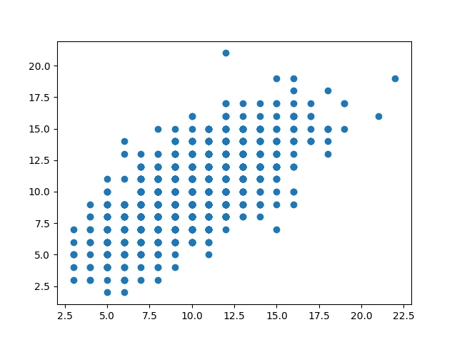
We can use the LVM formulation above to sample from arbitrary copulas. Below is an example in Python to sample two correlated Poisson variables.
import numpy as np
import matplotlib.pyplot as plt
from scipy.stats import norm
from scipy.stats import multivariate_normal
from scipy.stats import poisson

# Covariance of RVs
cov_mat = np.array([
	[1.0, 0.7],
	[0.7, 1.0]])

n = 1000
p = 2

# Generate latent variables
Z = multivariate_normal.rvs(mean=np.zeros(p), cov=cov_mat, size=n)

# Pass through standard normal CDF
Z_tilde = norm.cdf(Z)

# Inverse of observed distribution function
X = poisson.ppf(q=Z_tilde, mu=10)

# Plot
plt.scatter(X[:, 0], X[:, 1])
plt.show()
This code generates two correlated Poisson variables:
References
- Xue‐Kun Song, Peter. “Multivariate dispersion models generated from Gaussian copula.” Scandinavian Journal of Statistics 27.2 (2000): 305-320.
- Smith, Michael Stanley. “Bayesian approaches to copula modelling.” arXiv preprint arXiv:1112.4204 (2011).
- Dobra, Adrian, and Alex Lenkoski. “Copula Gaussian graphical models and their application to modeling functional disability data.” The Annals of Applied Statistics 5.2A (2011): 969-993.
- Professor Peter Bloomfield’s lecture slides.