Andy Jones
Gaussian copulas and the Global Financial Crisis
\(\DeclareMathOperator*{\argmin}{arg\,min}\) \(\DeclareMathOperator*{\argmax}{arg\,max}\)
The Global Financial Crisis in the late 2000s had complex causes, but a prominent theme among them stands out: many risky, correlated assets collapsed all at once.
Most financial assets and metrics – stock prices, inflation rates, risk measures, etc. – exhibit some amount of correlation with other, similar metrics. For example, stock prices exhibit correlation with one another (both positive and negative) during normal times.
However, the level of correlation between assets/securities can change dramatically depending on the macro-level state of the economy or industry. It’s important to not only examine and model these correlations when the economy is functioning normally, but also when the economy is in an unlikely, extreme state – a “tail event” in probability terms. When extreme values of financial metrics and prices are observed, the correlation structure can change dramatically. For example, during economic recessions, stock prices tend to be unusually correlated with one another as they all turn downward.
Most statistical models focus on explaining the “normal” or “typical” state of a phenomenon, while focusing less on modeling less likely events. This approach is reasonable for many settings where extreme events are not very impactful. However, for settings in which extreme events can pose a substantial harm, it is vital to model these outliers. In the economy, these tail events can often pose a systemic risk – meaning that even if they happen just once, it could cause a broad collapse. When a large financial institution, like a bank, is exposed to these assets without properly accounting for the tail risk, this poses an existential risk.
“The formula that killed Wall Street”
In 2009, Wired published an article titled “Recipe for Disaster: The Formula That Killed Wall Street”. The author, Felix Salmon, investigates the statistical methods used by large American banks and credit rating agencies to price mortgage-backed securities and collateralized debt obligations.
The article zeros in on one model in particular: the Gaussian copula. The basic idea behind copulas is that they can model joint distributions of arbitrary random variables. To define a copula-based model, all we need to know is the marginal distributions of each random variable and the level of correlation between the random variables. Copulas are attractive because they provide a straightforward, out-of-the-box way to model multiple correlated random variables that may not have a natural multivariate distribution.
While copula models have been around since the 1950s, it wasn’t until the early 2000s that they became popular in financial applications. Naturally, copulas are attractive tools for modeling multiple correlated financial assets. One of the first practitioners to propose a copula model for understanding credit risk was David Li. In 2000, Li published a paper proposing a statistical model for understanding risk of default and the correlation between the default risks across multiple loans.
The core of Li’s model was a Gaussian copula, which was used to model the correlation between the risk levels of multiple asset-backed securiites. However, as we will explore in more detail below, the Gaussian copula fails to correctly model extreme events. In particular, it has zero “tail dependence” – meaning that the model’s prediction of assets’ correlation with one another vanishes during extreme periods. For this reason, the Gaussian copula modeling approach proved to be inaccurate and disastrous for modeling credit risk.
The credit rating agencies and large banks used Li’s model (or a variant of it) to assign risk scores to different loans. Unfortunately, the model didn’t properly account for the situation in which a large majority of the loans go bad all at once – a tail event. In reality, the default risks of asset-backed securities exhibit strong correlation in the tails (especially the lower tails) because they’re all subject to the same macroeconomic factors. If the economy enters a recession, there is a spike in all of the securities’ probability of default.
However, under the Gaussian copula model, it is nearly impossible to have all of the securities default together. This means that the credit rating agencies and banks were overly optimistic about how much risk they could take on through asset-backed securities, believing that there was little chance of a broad collapse.
More broadly, banks administering mortgages must think carefully about which loans to extend in order to keep the overall risk of default at a manageable level. A bank may be able to tolerate a small percentage of their mortgages defaulting, but they want to make sure they avoid a situation where a large chunk of them default.
A key part of modeling this risk is accounting for these “extreme” scenarios. In statistics and probability, the field of modeling unlikely events that occur on the tails of probability distributions is called extreme value theory.
Below, we walk through a toy example of modeling credit risk, introducing copulas along the way.
A motivating example
Suppose Alice and Bob both take out mortgages through the same bank. Each homebuyer has a nonzero probability of defaulting on their loan; in other words, there’s a chance that each of them won’t be able to pay back their mortgage at some point, making the bank lose money on the loan.
Alice and Bob’s risks of defaulting depend on two types of factors:
- Their individual financial statuses (financial stability, employment status, credit score, etc.), which only affect each person’s own probability of default;
- Macroeconomic factors (inflation, interest rates, wars, etc.), which affect both homebuyers’ chances of default.
To account for the first type of factors, we can model Alice and Bob’s individual credit risks as univariate random variables. In this post (following Li’s modeling approach), we’ll model each person’s “time-until-default”, which is a random variable representing the number of years before they default on their loan.
Let $T_A, T_B \in \mathbb{R}_+$ be random variables representing the times-until-default for Alice and Bob, respectively. We will assume these RVs follow exponential distributions,
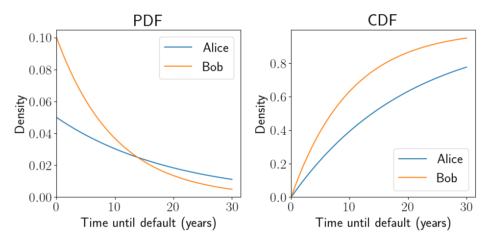
\[T_A \sim \text{Exp}(\lambda_A),~~~T_B \sim \text{Exp}(\lambda_B),\]where $\lambda_A$ and $\lambda_B$ are parameters controlling the shape of the distributions. In this example, we assume $\lambda_A = 1/20$ and $\lambda_B = 1/10,$ implying that Bob’s mortgage is at a higher risk of default than Alice’s (i.e., his time-until-default is generally sooner).
Recall that the PDF and CDF for the exponential distribution are given by
\[f(x; \lambda) = \lambda e^{-\lambda x},~~~F(x; \lambda) = 1 - e^{-\lambda x}.\]Below are plots of the PDFs and CDFs for Alice and Bob’s times-until-default:

We now have a model for Alice and Bob’s individual credit risk, but we haven’t specified a joint model that describes the level of correlation between their credit risks (the second set of factors above). This correlation must be taken into account when modeling risk of default. For example, if Alice defaults on her loan after one year, our model should raise Bob’s probability of default because he is exposed to many of the same macroeconomic factors as Alice.
We next introduce copulas, which can be used to specify a joint model.
Copulas
A copula is a multivariate CDF where each constituent random variable has a marginal distribution that is uniform. Specifically, a $p$-variate copula $C$ is a function $C : [0, 1]^p \to [0, 1]$ that maps a set of $p$ uniformly distributed random variables to a cumulative density.
For variables that are not intrinsically uniformly distributed, their CDFs can be applied before passing them through the copula function to make them uniform. Consider random variables $X_1, \dots, X_p$ with respective CDFs $F_1, \dots, F_p.$ Then we can model their joint distribution with a copula as follows:
\[C(u_1, \dots, u_p) = C(F_1(X_1), \dots, F_p(X_p)),\]where $F_j(X_j) \sim \text{Unif}(0, 1)$ for $j = 1, \dots, p$ by the definition of a CDF.
Several forms for the copula function $C$ have been proposed, one of which we will briefly explore below.
The Gaussian copula
The most popular variant of copula is the Gaussian copula. The Gaussian copula simply uses the univariate Gaussian inverse CDF $\Phi^{-1} : [0, 1] \to \mathbb{R}$ to make each marginal distribution Gaussian, and then uses the multivariate Gaussian CDF $\Phi_\Sigma : \mathbb{R}^p \to [0, 1]$ to model the correlation between the variables. The multivariate Gaussian CDF $\Phi_\Sigma$ is parameterized by a correlation matrix $\Sigma \in [-1, 1]^{p \times p}$ that describes the variables’ pairwise correlations. The full copula function is given by
\begin{align} C(u_1, \dots, u_p) &= C(F_1(X_1), \dots, F_p(X_p)) \\ &= \Phi_\Sigma(\Phi^{-1}(F_1(X_1)), \dots, \Phi^{-1}(F_p(X_p))). \end{align}
The Gaussian copula is attractive for its tractability and the community’s general familiarity with the multivariate Gaussian family.
Tail dependence
There are many ways to mathematically describe the relationship and dependence between two random variables. The most standard way is to use measures of correlation (e.g., Pearson correlation), which measure the overall linear relationship between the two RVs’ distributions. For example, in the Gaussian copula above, the matrix $\Sigma$ captures the correlational dependence between variables. Other measures of dependence focus on particular aspects of the distribution.
In extreme value theory, one type of dependence is particularly important: tail dependence. Intuitively, measures of tail dependence describe how strongly two distributions are related to one another in their tails, rather than across the entire distribution. In some cases the level of correlation between two random variables can be drastically different in their tails compared to the global dependence between them.
To give a more technical definition of tail dependence, let $X$ and $Y$ be two random variables whose CDFs are given by $F$ and $G,$ respectively. Define $U = F(X)$ and $V = G(Y).$ We can then define tail dependence coefficients for both the lower and upper tails of the distributions. The lower tail dependence coefficient $\lambda_L$ is defined as
\[\lambda_L = \lim_{u \downarrow 0} \mathbb{P}(V < u | U = u) + \mathbb{P}(U < u | V = u).\]Similarly, the upper tail dependence coefficient is defined as
\[\lambda_U = \lim_{u \uparrow 1} \mathbb{P}(V > u | U = u) + \mathbb{P}(U > u | V = u).\]When $U$ and $V$ are exchangeable, these coefficients can be simplified as
\[\lambda_L = 2 \lim_{u \downarrow 0} \mathbb{P}(V < u | U = u),~~\lambda_U = 2 \lim_{u \uparrow 1} \mathbb{P}(V > u | U = u).\]Intuitively, the lower and upper tail dependence coefficients measure how likely it is that one random variable takes on an extreme value given that we observed an extreme value for the other random variable. These coefficients take values in $[0, 1],$ where higher values imply stronger tail dependence.
Tail dependence under the Gaussian copula
We next study tail dependence in the Gaussian copula, showing that its tail dependence coefficients are zero.
Consider two standard Gaussian random variables, $X, Y \sim \mathcal{N}(0, 1)$ whose correlation is given by $\rho,$ where $-1 \leq \rho \leq 1.$ Writing $X$ and $Y$ as a bivariate vector, we have
\[\begin{bmatrix} X \\ Y \end{bmatrix} \sim \mathcal{N}\left( \begin{bmatrix} 0 \\ 0 \end{bmatrix}, \begin{bmatrix} 1 & \rho \\ \rho & 1 \end{bmatrix} \right).\]Letting $V = \Phi(Y)$ and $U = \Phi(X)$ and relying on the fact that $X$ and $Y$ are exchangeable, we can write the upper tail dependence coefficient as
\[\lambda_U = 2 \lim_{u \uparrow 1} \mathbb{P}(V > u | U = u) = 2 \lim_{u \uparrow 1} \mathbb{P}(\Phi(Y) > u | \Phi(X) = u),\]where $\Phi(\cdot)$ is the standard normal CDF. Applying the inverse CDF to both sides of the inequality, we have
\begin{align} \lambda_U &= 2 \lim_{\Phi^{-1}(u) \to \Phi^{-1}(1)} \mathbb{P}(Y > \Phi^{-1}(u) | X = \Phi^{-1}(u)) \\ &= 2 \lim_{x \to \infty} \mathbb{P}(Y > x | X = x), \end{align}
where $\Phi(x) = u.$
Using well-known properties of the multivariate Gaussian, we know that the conditional distribution of $Y$ given $X$ is
\[Y | (X = x) \sim \mathcal{N}(\rho x, 1 - \rho^2).\]For simplicity, define a new random variable $T$ as $T = \frac{Y - \rho x}{\sqrt{1 - \rho^2}}.$ Then we have
\[T | (X = x) \sim \mathcal{N}(0, 1).\]We can then plug this into the definition of the tail dependence coefficient and simplify:
\begin{align} \mathbb{P}(Y > x | X = x) &= 1 - \mathbb{P}(Y \leq x | X = x) & \text{“Survival function”} \\ &= 1 - \mathbb{P}\left(T \leq \frac{x - \rho x}{\sqrt{1 - \rho^2}} | X = x\right) \\ &= 1 - \Phi\left(\frac{x(1 - \rho)}{\sqrt{1 - \rho^2}}\right) \\ &= 1 - \Phi\left(\frac{x(1 - \rho)}{\sqrt{(1 - \rho) (1 + \rho)}}\right) & \text{Multiply by $\frac{\sqrt{1 - \rho}}{\sqrt{1 - \rho}}$} \\ &= 1 - \Phi\left(\frac{x \sqrt{1 - \rho}}{\sqrt{1 + \rho}}\right). \end{align}
Clearly, if $\rho=1$ (i.e., $X$ and $Y$ are perfectly correlated), then we have
\begin{align} \lambda_U &= 2 \lim_{x \to \infty} \mathbb{P}(Y > x | X = x) \\ &= 2 - 2 \Phi(0) \\ &= 2 - 2 \cdot 0.5 \\ &= 1, \end{align}
implying that $X$ and $Y$ have maximal tail dependence. For $\rho < 1,$ we have
\begin{align} \lambda_U &= 2 \lim_{x \to \infty} \mathbb{P}(Y > x | X = x) \\ &= 2 - 2 \cdot \Phi(\infty) \\ &= 2 - 2 \cdot 1 \\ &= 0, \end{align}
implying that $X$ and $Y$ have no tail dependence.
A simple example demonstrating tail dependence
Let’s continue our example above in which Alice and Bob are new homeowners who have just taken out mortgages. Let’s model their default risks as follows.
Now that we have a model for the marginal distributions of Alice and Bob’s times-until-default, we need a model for the correlation between them. For this, let’s experiment with two different types of copulas: the Gaussian copula (which was used in David Li’s paper) and the $t$-copula with two degrees of freedom. Unlike the Gaussian copula, the $t$-copula has tail dependence.
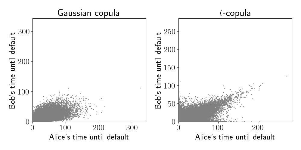
Below, we generate 100,000 samples from each of these models.

We can already see that the $t$-copula has a strong correlation in its upper tails (visible via the top right spike in the right panel). There is also strong correlation in its lower tails, although this is less visible due to the crowding of points. On the other hand, the samples from the Gaussian copula resemble a bivariate normal distribution, with correlation in its center.
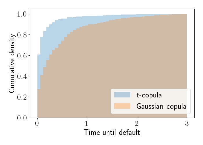
To get another view of how these models behave in their tails, let’s check numerically for measures of tail dependence. Below, we compute the empirical conditional CDF for each of the models for all samples with a time-until-default of at most three years. Specifically, we first subset Bob’s samples to the subset where Alice’s corresponding time-until-default is at most 0.01. We then compute the empirical CDF of Bob’s times-until-default. The CDFs are shown below.

We see that the $t$-copula has more mass on smaller times-until-default compared to the Gaussian copula. In fact, the Gaussian copula’s mass will eventually go to zero at the left end of the plot.
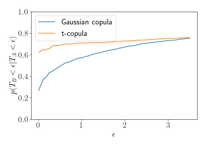
Extending this analysis, we can compute an empirical version of the lower tail dependence coefficient. We do so by computing an empirical average:
\[\widehat{\lambda}_L = \frac{1}{n_\epsilon} \mathbb{I}\left\{T_B < \epsilon | T_A < \epsilon\right\},\]where $n_\epsilon = \mathbb{I}\left\{ T_A < \epsilon \right\}.$ We compute this for a range of values for $\epsilon$ for each model. The results are below.

We see that the left side of the plot begins to numerically recover the fact that the Gaussian copula has no tail dependence, as the blue line trends toward zero. The $t$-copula, on the other hand, converges to a nonzero tail dependence coefficient.
Code
See this Jupyter notebook for the code used in this post.
References
- Li, David X. “On default correlation: A copula function approach.” The Journal of Fixed Income 9.4 (2000): 43-54.
- Embrechts, Paul, Filip Lindskog, and Alexander McNeil. “Modelling dependence with copulas.” Rapport technique, Département de mathématiques, Institut Fédéral de Technologie de Zurich, Zurich 14 (2001): 1-50.
- Watts, Samuel. “The Gaussian copula and the financial crisis: A recipe for disaster or cooking the books?.” (2016).