Andy Jones
Convex cones and positive definite matrices
\(\DeclareMathOperator*{\argmin}{arg\,min}\) \(\DeclareMathOperator*{\argmax}{arg\,max}\)
In this post, we review cones, convex cones, and their relationship to positive definite matrices.
Cones
A cone is a vector space that is closed under scalar multiplication. Notationally, we say that a set $\mathcal{C}$ is a cone if, for any $\theta \in \mathbb{R}$ and for every $\mathbf{x} \in \mathcal{C}$, it holds that $\theta \mathbf{x} \in \mathcal{C}.$
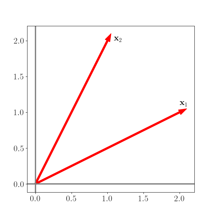
To visualize a cone in two dimensions, consider the two vectors $\mathbf{x}_1 = [2, 1]^\top$ and $\mathbf{x}_2 = [1, 2]^\top.$ We plot these vectors below.
Now let’s consider the span of these two vectors (which is a vector space). Recall that the span of these two vectors is given by
\[\text{span}(\{\mathbf{x}_1, \mathbf{x}_2\}) = \left\{ a_1 \mathbf{x}_1 + a_2 \mathbf{x}_2 \right | a_1, a_2 \in \mathbb{R}\}.\]We can visualize the span below.
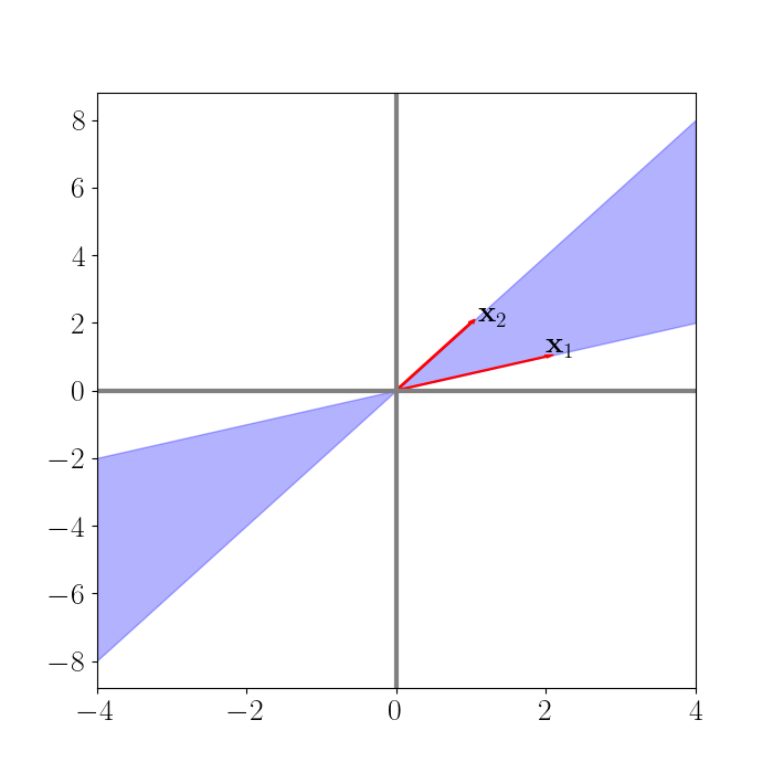
Visually, we can notice that, on either side of the y-axis, this figure looks like a cone. Across the entire plot, it appears more like an hourglass (and this is characteristic of cones). To algebraically check if this vector space is a cone, consider any $a_1, a_2 \in \mathbb{R}.$ Let’s check if the definition of a cone holds. For any $\theta \in \mathbb{R},$ we have:
\begin{align} \theta \left(a_1 \mathbf{x}_1 + a_2 \mathbf{x}_2\right) &= \theta a_1 \mathbf{x}_1 + \theta a_2 \mathbf{x}_2 \\ &= b_1 \mathbf{x}_1 + b_2 \mathbf{x}_2, \end{align}
where $b_1 = \theta a_1,$ $b_2 = \theta a_2,$ and $b_1, b_2 \in \mathbb{R}.$ Thus, this linear combination still resides in $\text{span}(\{\mathbf{x}_1, \mathbf{x}_2\})$, which implies that the vector space is closed under scalar multiplication and is a cone.
Convex cones
A convex cone is a special type of cone. In particular, a convex cone is a cone that is closed under linear combinations with positive coefficients. Notationally, we say that a set $\mathcal{C}$ is a convex cone if, for any $\theta_1, \theta_2 \in \mathbb{R}_+$ and for every $\mathbf{x}_1, \mathbf{x}_2 \in \mathcal{C}$, it holds that $\theta_1 \mathbf{x}_1 + \theta_2 \mathbf{x}_2 \in \mathcal{C}.$
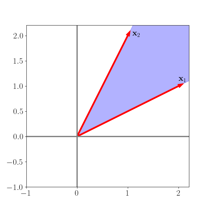
Continuing with our two-dimensional example above, consider all linear combinations of $\mathbf{x}_1$ and $\mathbf{x}_2$ with positive coefficients. This set of linear combinations will form a convex cone that resembles the cone we encountered above, but now only includes the portion of the cone to the right of the y-axis. We plot the convex cone defined by the positive-coefficient linear combinations of $\mathbf{x}_1$ and $\mathbf{x}_2$ below.
A key relationship between matrices and convex cones is that the set of all positive definite (PD) matrices is a cone. We can easily show this algebraically. Recall the definition of a PD matrix $\mathbf{X} \in \mathbb{R}^{n \times n}:$ $\mathbf{X}$ is PD if, for any $\mathbf{z} \in \mathbb{R}^n,$ it holds that $\mathbf{z}^\top \mathbf{X} \mathbf{z} > 0.$
We can check that the definition of a convex cone holds for the set of PD matrices. Consider two PD matrices $\mathbf{X}_1$ and $\mathbf{X}_2$, and let $\theta_1, \theta_2 \in \mathbb{R}_+$ be any two positive scalars. We can check if the linear combination $\theta_1 \mathbf{X}_1 + \theta_2 \mathbf{X}_2$ is still positive definite. Again, let $\mathbf{z} \in \mathbb{R}^n.$ Then we have:
\begin{align} \mathbf{z}^\top \left(\theta_1 \mathbf{X}_1 + \theta_2 \mathbf{X}_2\right) \mathbf{z} &= \theta_1 \mathbf{z}^\top \mathbf{X}_1 \mathbf{z} + \theta_2 \mathbf{z}^\top \mathbf{X}_2 \mathbf{z} \\ &= \theta_1 b_1 + \theta_2 b_2, \end{align}
where we know $b_1, b_2 > 0$ due to the definition of PD matrices. Since $\theta_1$ and $\theta_2$ are also positive, we can conclude that this linear combination is also PD, and thus that the set of PD matrices forms a convex cone.
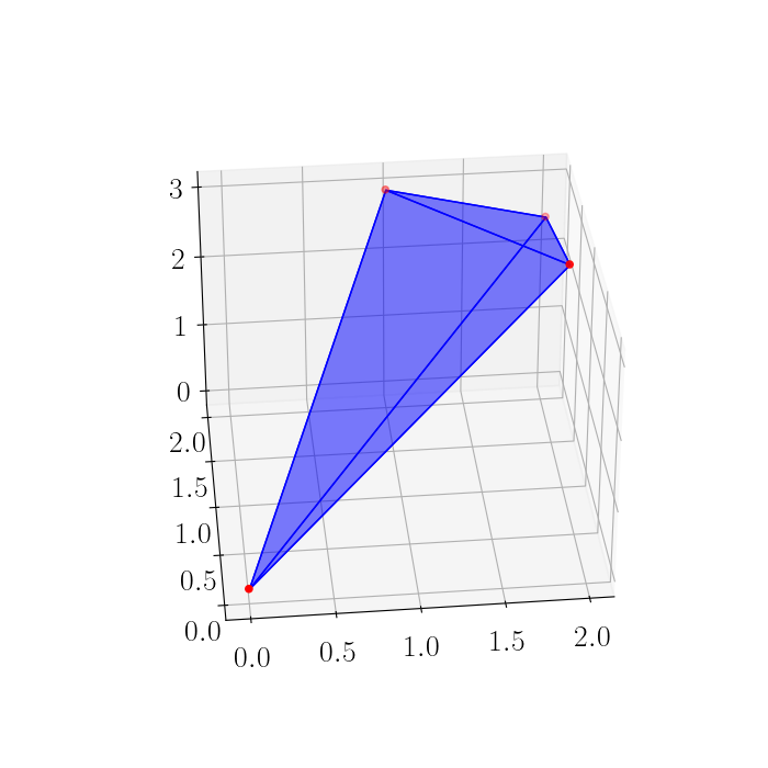
In higher dimensions, the finitely-generated convex cones we considered above form polyhedra. For example, in three dimensions we can extend our example above to consider the convex cone generated by three vectors, $\mathbf{x}_1 = [1, 2, 3], \mathbf{x}_2 = [2, 1, 3], \mathbf{x}_3 = [2, 2, 2.5].$ The polyhedron defined by this convex cone is below.
Significance in statistics and optimization
PD matrices, and thus convex cones, are important in many statistical applications because covariance matrices are a central quantity in many multivariate statistical models. A covariance matrix is a symmetric and PD matrix that describes the (co)variance between each pair of random variables.
In optimization, the class of conic optimization problems is quite large, and is a generalization of linear and semidefinite programming problems.