Convergence in probability vs. almost sure convergence

When thinking about the convergence of random quantities, two types of convergence that are often confused with one another are convergence in probability and almost sure convergence. Here, I give the definition of each and a simple example that illustrates the difference. The example comes from the textbook Statistical Inference by Casella and Berger, but I’ll step through the example in more detail.

Definitions

A sequence of random variables $X_1, X_2, \dots X_n$ converges in probability to a random variable $X$ if, for every $\epsilon > 0$,

\begin{align}\lim_{n \rightarrow \infty} P(\lvert X_n - X \rvert < \epsilon) = 1.\end{align}

A sequence of random variables $X_1, X_2, \dots X_n$ converges almost surely to a random variable $X$ if, for every $\epsilon > 0$,

\begin{align}P(\lim_{n \rightarrow \infty} \lvert X_n - X \rvert < \epsilon) = 1.\end{align}

As you can see, the difference between the two is whether the limit is inside or outside the probability. To assess convergence in probability, we look at the limit of the probability value $P(\lvert X_n - X \rvert < \epsilon)$, whereas in almost sure convergence we look at the limit of the quantity $\lvert X_n - X \rvert$ and then compute the probability of this limit being less than $\epsilon$.

Example

Let’s look at an example of sequence that converges in probability, but not almost surely. Let $s$ be a uniform random draw from the interval $[0, 1]$, and let $I_{[a, b]}(s)$ denote the indicator function, i.e., takes the value $1$ if $s \in [a, b]$ and $0$ otherwise. Here’s the sequence, defined over the interval $[0, 1]$:

\begin{align}X_1(s) &= s + I_{[0, 1]}(s) \\ X_2(s) &= s + I_{[0, \frac{1}{2}]}(s) \\ X_3(s) &= s + I_{[\frac{1}{2}, 1]}(s) \\ X_4(s) &= s + I_{[0, \frac{1}{3}]}(s) \\ X_5(s) &= s + I_{[\frac{1}{3}, \frac{2}{3}]}(s) \\ X_6(s) &= s + I_{[\frac{2}{3}, 1]}(s) \\ &\dots \\ \end{align}

As you can see, each value in the sequence will either take the value $s$ or $1 + s$, and it will jump between these two forever, but the jumping will become less frequent as $n$ become large. For example, the plot below shows the first part of the sequence for $s = 0.78$. Notice that the $1 + s$ terms are becoming more spaced out as the index $n$ increases.

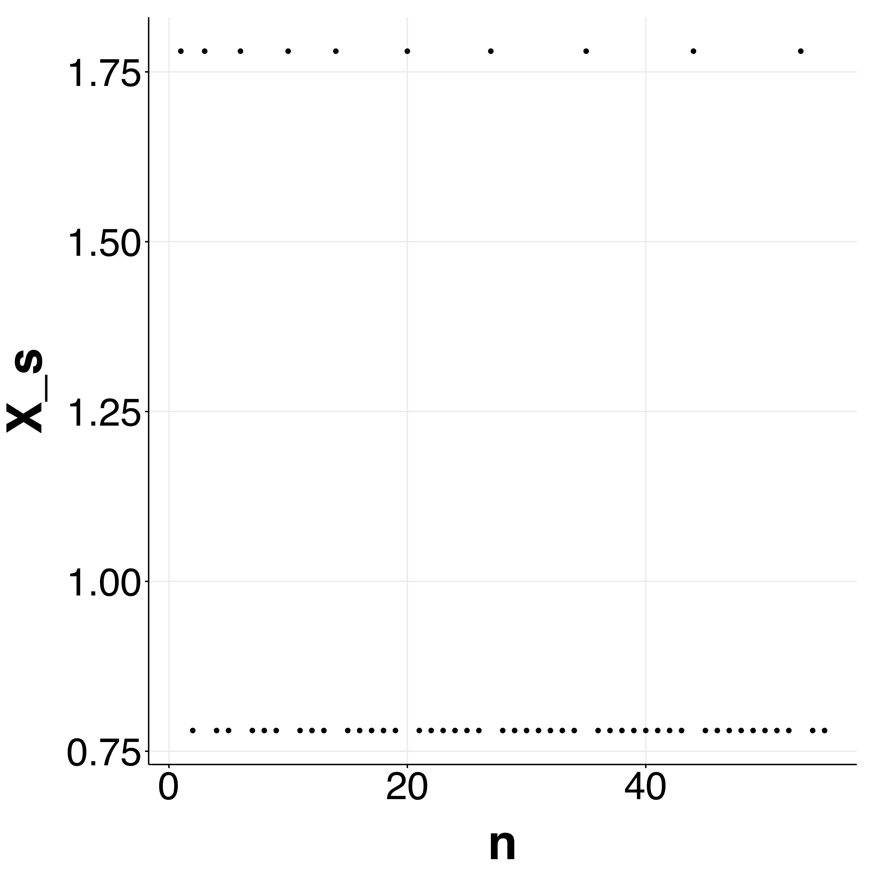
We can explicitly show that the “waiting times” between $1 + s$ terms is increasing:

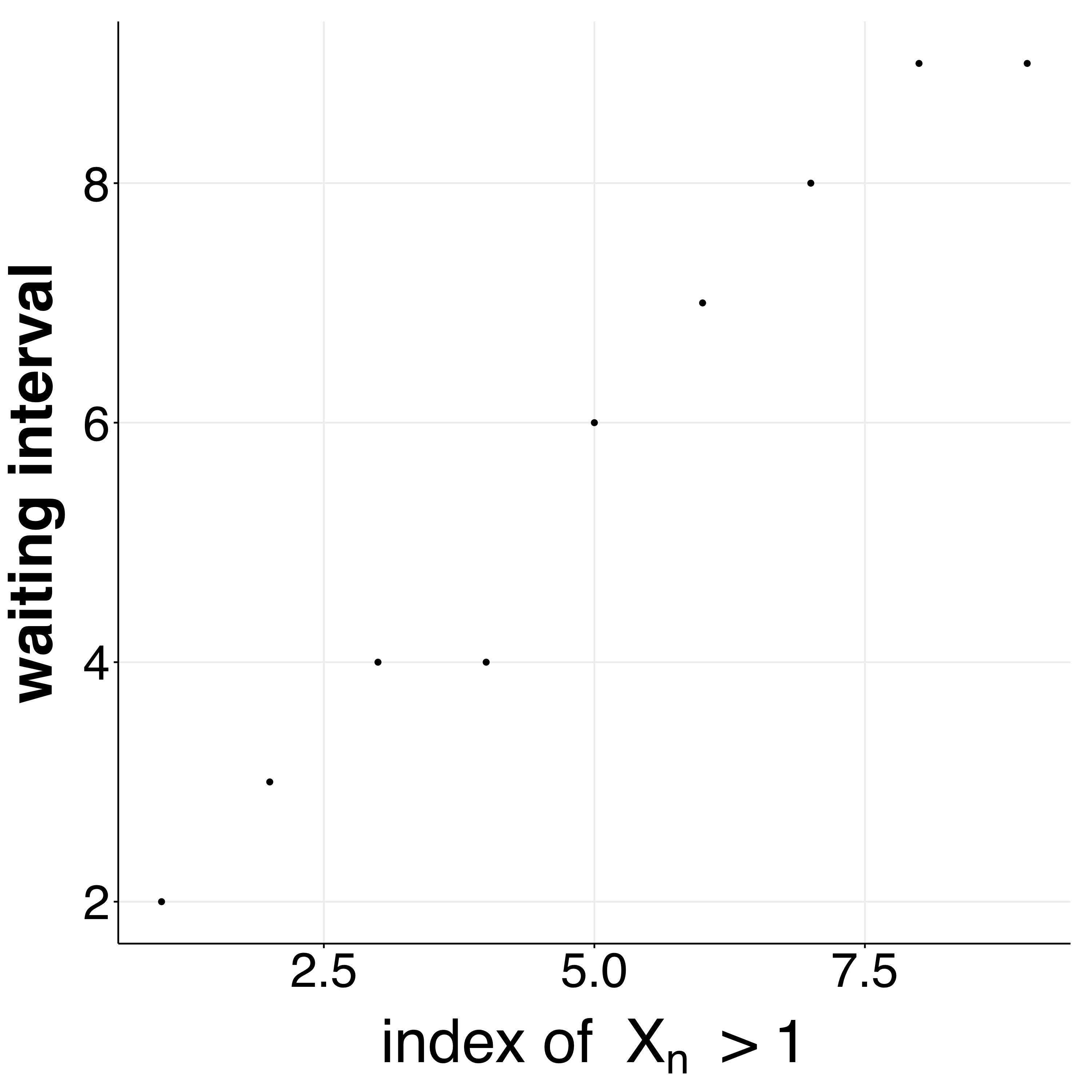
Now, consider the quantity $X(s) = s$, and let’s look at whether the sequence converges to $X(s)$ in probability and/or almost surely.

For convergence in probability, recall that we want to evaluate whether the following limit holds

\begin{align}\lim_{n \rightarrow \infty} P(\lvert X_n(s) - X(s) \rvert < \epsilon) = 1.\end{align}

Notice that the probability that as the sequence goes along, the probability that $X_n(s) = X(s) = s$ is increasing. In the plot above, you can notice this empirically by the points becoming more clumped at $s$ as $n$ increases. Thus, the probability that the difference $X_n(s) - X(s)$ is large will become arbitrarily small. Said another way, for any $\epsilon$, we’ll be able to find a term in the sequence such that $P(\lvert X_n(s) - X(s) \rvert < \epsilon)$ is true. We can conclude that the sequence converges in probability to $X(s)$.

Now, recall that for almost sure convergence, we’re analyzing the statement

\begin{align}P(\lim_{n \rightarrow \infty} \lvert X_n - X \rvert < \epsilon) = 1.\end{align}

Here, we essentially need to examine whether for every $\epsilon$, we can find a term in the sequence such that all following terms satisfy $\lvert X_n - X \rvert < \epsilon$. However, recall that although the gaps between the $1 + s$ terms will become large, the sequence will always bounce between $s$ and $1 + s$ with some nonzero frequency. Thus, the probability that $\lim_{n \rightarrow \infty} \lvert X_n - X \rvert < \epsilon$ does not go to one as $n \rightarrow \infty$, and we can conclude that the sequence does not converge to $X(s)$ almost surely.

Strong and weak laws of large numbers

An important application where the distinction between these two types of convergence is important is the law of large numbers. Recall that there is a “strong” law of large numbers and a “weak” law of large numbers, each of which basically says that the sample mean will converge to the true population mean as the sample size becomes large. Importantly, the strong LLN says that it will converge almost surely, while the weak LLN says that it will converge in probability. We have seen that almost sure convergence is stronger, which is the reason for the naming of these two LLNs.

Conclusion

In conclusion, we walked through an example of a sequence that converges in probability but does not converge almost surely. In general, almost sure convergence is stronger than convergence in probability, and a.s. convergence implies convergence in probability.

References

Casella, G. and R. L. Berger (2002): Statistical Inference, Duxbury.