Conjugate gradients

\(\DeclareMathOperator*{\argmin}{arg\,min}\) \(\DeclareMathOperator*{\argmax}{arg\,max}\)

Efficiently solving large linear systems of equations is a core problem in optimization. These problems take the form of solving for $\mathbf{x} \in \mathbb{R}^d$ that satisfies

where $\mathbf{A} \in \mathbb{R}^{d \times d}$ and $\mathbf{b} \in \mathbb{R}^d$ are known. Conjugate gradient descent is a method for estimating these solutions when $\mathbf{A}$ is symmetric and positive definite. These problems are ubiquitous in statistics and machine learning. Below we provide two motivating examples, and then proceed to describe conjugate gradients and conjugate gradient descent.

Quadratic loss functions

One situation that arises frequently that requires solving linear systems is the minimization of a quadratic function. Specifically, consider the following optimization program:

where again $\mathbf{A}$ and $\mathbf{b}$ are known. The gradient with respect to $\mathbf{x}$ is

In order to minimize our original quadratic function, we’d like to find the zeros of this linear equation. Equivalently, we would like to find $\mathbf{x}$ such that $\mathbf{A}\mathbf{x} = \mathbf{b}.$

Gaussian likelihoods

When working with Gaussian statistical models, we often encounter log likelihoods of the form

where $\mathbf{A}$ is the covariance matrix of a $d$-dimensional multivariate Gaussian $\mathcal{N}(\mathbf{0}, \mathbf{A})$ in this case. Computing the inverse $\mathbf{A}^{-1}$ will require $O(d^3)$ computation in general. However, if we instead try to directly estimate $\mathbf{A}^{-1} \mathbf{b}$, we can see this is a linear system. In particular, the problem is to find $\mathbf{x}$ such that

By using faster methods to estimate this linear system, we can save computation time.

Gradient descent

Gradient descent (GD) is a central building block for lots of gradient-based optimization algorithms, including conjugate gradient descent. Recall that the basic idea behind GD is to take a step in the direction of the negative gradient at each iteration.

Let $f(\mathbf{x}) : \mathbb{R}^d \rightarrow \mathbb{R}$ be our loss function that we wish to minimize. Given a current estimate $\mathbf{x}_t$ on the $t$th iteration, GD takes the following update:

where $\alpha_t$ is a learning rate parameter (which may also be constant on each iteration). We can continue to take these steps until we’re satisfied with the result. A common way of assessing convergence is to track the reduction in the loss between iterations, and to stop when this reduction falls below some threshold:

Conjugate gradient descent

Conjugate gradient descent (CGD) adapts the idea of GD to better accommodate the geometry of the objective function. Rather than taking a step in the direction of the negative gradient locally, CGD constrains each step to be orthogonal to the previous ones.

Specifically, CGD accounts for the second-order curvature of the loss landscape. In our quadratic loss function above, this second-order geometry is encoded in $\mathbf{A}.$ We’ll first review the intuition behind conjugate vectors accounting for $\mathbf{A}$, and then describe CGD.

Conjugacy

Two vectors $\mathbf{u}$ and $\mathbf{v}$ are said to be $\mathbf{A}$-orthogonal or “conjugate with respect to $\mathbf{A}$” if

In other words, $\mathbf{u}$ and $\mathbf{v}$ are orthogonal after accounting for the structure imposed by $\mathbf{A}.$ Note that if $\mathbf{A} = \mathbf{I}$, where $\mathbf{I}$ is the identity matrix, we recover the classic Euclidean notion of orthogonality.

To visualize this notion of orthogonality/conjugacy, consider the animation below. Each plot shows the contours for a quadratic loss function for varying values of $\mathbf{A}$. On top of the contours we plot one vector $(-7, 0)^\top$ in black whose starting point is $(7, 7)^\top.$ We also plot a vector that is $\mathbf{A}$-orthogonal to the black vector in red.

We can see that when $\mathbf{A} = \mathbf{I}$ in the middle of the animation, we recover the traditional notion of orthogonality (a $90^{\circ}$ angle between the vectors). However, for other values of $\mathbf{A}$, orthogonality takes a different form that accounts for the stretching of the contours.

Conjugate gradient descent: the algorithm

CGD requires the direction of each step to be $\mathbf{A}$-orthogonal to each of the previous steps. In particular, CGD takes a step in the direction of the negative gradient, but first requires that we “project out” the previous directions. Let $\mathbf{g}_t = \nabla_{\mathbf{x}} f(\mathbf{x})$ be the gradient at the current step. In the traditional Euclidean sense, the projection of $\mathbf{g}_t$ onto a previous step direction $\mathbf{p}_{t^\prime}$ is

However, in CGD we will adapt this projection slightly in order to account for $\mathbf{A}$. In particular, we’ll take the projection to be

Our update on the $t$th step will be the gradient with these projections subtracted out. Namely:

Our update will then be a step of length $\alpha_t$ in this direction:

Notice that, because of our conjugacy constraints, the algorithm will require at most $d$ steps, where $d$ is the dimension of the problem.

The final piece is to find the best step size $\alpha_t.$ We can do this by directly minimizing $f$:

\begin{align} \alpha_t^\star &= \argmin_{\alpha_t} f(\mathbf{x}_t + \alpha_t \mathbf{p}_t) \\ &= \argmin_{\alpha_t} \frac12 (\mathbf{x}_{t - 1} + \alpha_t \mathbf{p}_t)^\top \mathbf{A} (\mathbf{x}_t + \alpha_t \mathbf{p}_t) - (\mathbf{x}_t + \alpha_t \mathbf{p}_t)^\top \mathbf{b} \\ &= \argmin_{\alpha_t} \alpha_t \mathbf{p}_t^\top \mathbf{A} \mathbf{x}_t + \frac12 \alpha_t^2 \mathbf{p}_t^\top \mathbf{p}_t - \alpha_t \mathbf{p}_t^\top \mathbf{b}.\end{align}

Taking the derivative with respect to $\alpha_t$ and setting it to zero, we have

Solving for $\alpha_t^\star$, this implies that

Example

Let’s see a simple example. Suppose we want to solve for $\mathbf{x}$ such that $\mathbf{A} \mathbf{x} = \mathbf{b}$, where

Suppose our starting point is $x_0 = (8, 3)^\top,$ and we run both GD and CGD to find $\mathbf{x}^\star.$

Below is a simple Python function for running CGD. For simplicity, it assumes $\mathbf{b} = \mathbf{0}.$

def CGD(A):
    d = A.shape[0]                          # Dimension of problem
    xhat = np.random.normal(size=d)         # Starting point

    # Prepare for first step
    g = -A @ xhat                           # Compute gradient
    p = g                                   # First step is in direction of grad
    g_len = g.T @ g                         # For normalization

    # Start running CGD
    for ii in range(len(xhat)):
            Ap = A @ p
            alpha = g_len / (p.T @ A @ p)   # Step size
            step = alpha * p                # Combine direction and step size
            xhat += step                    # Take step
            g = g - alpha * A @ p
            g_len_new = g.T @ g
            p = g + (g_len_new / g_len) * p # Update p
            g_len = g_len_new

    return xhat

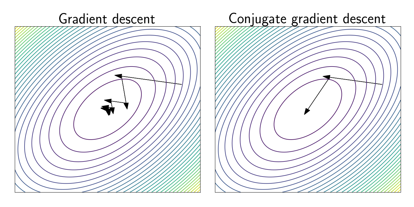
The left panel shows the steps taken by GD. We can see that GD criss-crosses back and forth across the loss landscape, eventually reaching the minimum after several steps.

The right panel shows CGD. We can see that the first step is identical to the first step of GD. This makes sense, as there are no orthogonality constraints on the first step. However, we see that the second step is different from GD. This arises becuase we have projected out the contribution from the direction of the first step. This leads us directly into the minimum in this case.

References

• Wikipedia page on conjugate gradients.
• Shewchuk, Jonathan Richard. “An introduction to the conjugate gradient method without the agonizing pain.” (1994): 1.