Andy Jones
The Concrete Distribution
The Concrete distribution is a relaxation of discrete distributions.
Here, we explain the motivation for relaxing discrete distributions and the properties of the Concrete distribution.
To start, note that the distribution was discovered simultaneously by Maddison et al. and Jang et al.. Below, I fluidly use terminology from both papers, focusing more on the core, shared ideas than either implementation in particular.
Reparameterization trick
The reparameterization ``trick’’ actually refers to a family of methods for sampling from a distribution using alternate parameterizations. Most commonly, it amounts to reparameterizing a random variable so that it’s described by a deterministic function that takes as input the distribution’s parameters and another random variable from a fixed distribution. This trick is useful for fitting certain statistical models using gradient descent.
Concretely, let’s say $z$ is a random variable drawn from a distribution $p_\theta$. The reparameterization trick seeks to find a function $g_\phi(\theta, \epsilon)$ such that if $\epsilon$ is randomly drawn from a fixed distribution, then the output of $g$ is a sample from $p_\theta$.
The most common example of the reparameterization trick uses the Gaussian distribution. Let $z \sim \mathcal{N}(\mu, \sigma^2)$. We can reparameterize this as \(\tilde{z} = \mu + \sigma \epsilon, \;\;\; \epsilon \sim \mathcal{N}(0, 1).\)
Since adding a constant to a Gaussian shifts its mean, and multiplying by a constant $c$ scales the variance by $c^2$, we have that $\tilde{z} \sim \mathcal{N}(\mu, \sigma^2)$.
There are many other instances of the reparameterization trick. In the paper that originally introduced it, the authors mention that there are three primary classes of distributions that are amenable to the trick:
- When the distribution has a tractable inverse CDF. In this case, we can use the inverse transform method.
- When the distribution is in the location-scale family. In this case, we can use the same approach as the Gaussian example above.
- When the distribution can be expressed as a composition of other random variables (e.g., a log-normal random variable is the exponential of a normal random variable).
Unfortunately, discrete random variables meet none of these criteria.
Concrete distribution
The concrete distribution relies on a reparameterization of the multinomial distribution – this trick is called the Gumbel max trick.
Suppose we want to sample from a multinomial with $k$ classes with associated probabilities $\pi_1, \dots, \pi_k$. The Gumbel max trick exploits the fact that the following quantity follows the distribution $\text{Mult}(\pi_1, \dots, \pi_k)$:
\[z = \text{arg}\max_{i \in [k]} \left[\log(\pi_i) + g_i\right], \;\;\; g_i \sim \text{Gumbel}(0, 1).\]In words, this means that if we add independent Gumbel noise to each of the class probabilities and take the arg-maximum, the output will have the desired multinomial distribution.
However, in the setting of optimization, this trick still isn’t differentiable with respect to the parameters (since the $\text{arg}\max$ operation isn’t differentable).
This is where the Concrete distribution comes into the picture. This distribution is a relaxation of the multinomial distribution, which is also differentiable with respect to its parameters.
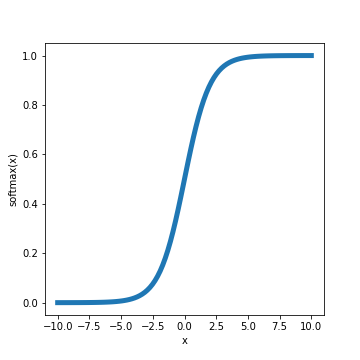
The easiest way to understand the Concrete distribution is as a relaxation of the Gumbel max trick itself: instead of taking the $\text{arg}\max$ above, we simply take the softmax. The softmax is a function $f : \mathbb{R}^k \mapsto \mathbb{R}^k$ whose $i$th output is defined as the following:
\[f(x_1, \dots, x_k)_i = \frac{\exp(x_i)}{\sum_j \exp(x_j)}\]The softmax function looks like this:
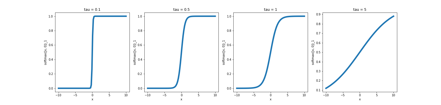
Often, a “temperature” parameter $\tau$ is included in the softmax function, which controls how steep the function is. The form of the function is then: \(f(x_1, \dots, x_k)_i = \frac{\exp(x_i / \tau)}{\sum_j \exp(x_j / \tau)}.\)
Plotting this function across different temperatures, we can see that it approaches a step function as the temperature decreases.
Now, if we combine our temperature-controlled softmax function with the Gumbel max trick, we can approximate the Multinomial with the following operation:
\[z_i = \frac{\exp\left\{(\log(\pi_i) + g_i) / \tau\right\}}{\sum_j \exp\left\{(\log(\pi_j) + g_j) / \tau\right\}}\]This is the sampling process for the Concrete distribution.
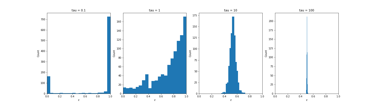
As a simple example, consider the case when we have just two classes $k=2$, and the class probabilities are $\pi_1 = 0.2, \pi_2 = 0.8$. If we sample from the Concrete distribution at varying temperatures and plot $z_1$ (the first element of the output vector), we see that the samples approach the discrete multinomial as the temperature decreases, and becomes more uniform at higher temperatures.
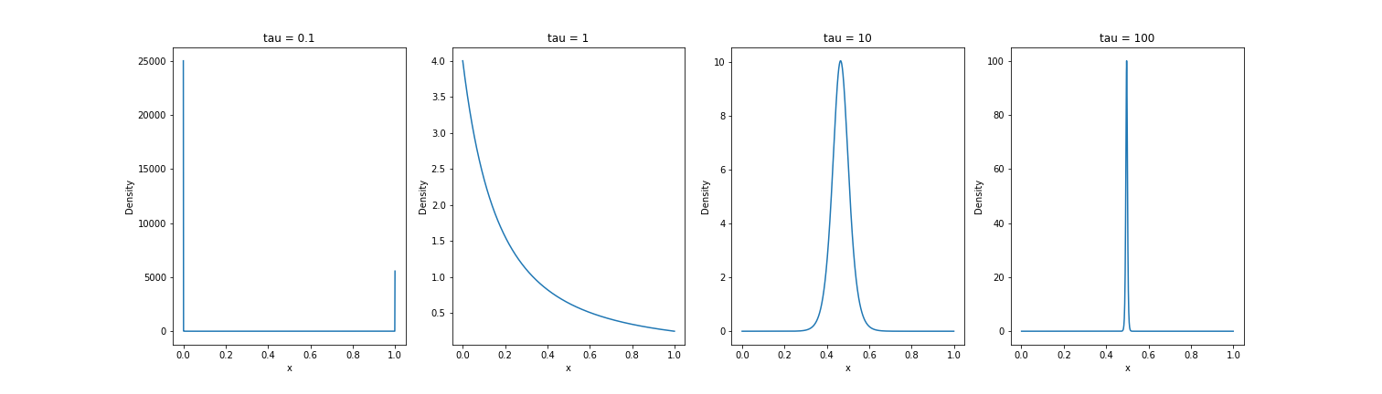
So far, we have just described the sampling procedure. But we can also define a proper probability density. The Concrete distribution is a two-parameter distribution with the following PDF:
\[p(x_1, \dots, x_k; \boldsymbol{\pi}, \tau) = \frac{\Gamma(k) \tau^{k-1}}{\left(\sum\limits_{i=1}^k \pi_i / y_i^\tau\right)^k} \prod\limits_{i=1}^k (\pi_i / y_i^{\tau + 1}).\]Plotting the density for $\pi_1 = 0.2, \pi_2 = 0.8$, we can see similar behavior as the temperature increases and decreases:
An application of the Concrete distribution: variational inference
One of the settings in which the reparameterization trick is most useful is variational inference. VI is a general approach to performing approximate posterior inference in statistical models that seeks to approximate a distribution $p(z | x)$ using another family of distributions $q(z | x)$.
Under the variational approach, the objective is to minimize the KL-divergence between the true posterior $p$ and the approximate posterior $q$. In turn, one typically seeks to maximize a lower bound on the log model evidence. This is called the evidence lower bound (ELBO) and is written as:
\[\log p(x) \geq \mathbb{E}_{q(z | x)} [-\log q(z | x) + \log p(x, z)] =: \mathcal{L}.\]In the seminal paper Auto-Encoding Variational Bayes, the authors found that this objective $\mathcal{L}$ could be maximized using stochastic gradient descent. To use SGD in this setting, one has to reparameterize the stochastic nodes.
In models with discrete latent variables, gradient descent was intractable because one could not use generic methods such as the inverse transform method to reparameterize the distributions (because it would not be differentiable).
This is where the benefit of the Concrete distribution arises: instead of directly using the desired discrete distribution, we can use the Concrete relaxation, which allows us to backpropagate gradients through the model.
References
Please note that the first two references (Maddison et al. and Jang et al.) simultaneously discovered this distribution and typically share credit in the literature. In this post, I used “Concrete distribution” as the default terminology but borrowed ideas and notation from both papers.
- Maddison, Chris J., Andriy Mnih, and Yee Whye Teh. “The concrete distribution: A continuous relaxation of discrete random variables.” arXiv preprint arXiv:1611.00712 (2016).
- Jang, Eric, Shixiang Gu, and Ben Poole. “Categorical reparameterization with gumbel-softmax.” arXiv preprint arXiv:1611.01144 (2016).
- Kingma, Diederik P., and Max Welling. “Auto-encoding variational bayes.” arXiv preprint arXiv:1312.6114 (2013).