Andy Jones
Classification and regression trees
\(\DeclareMathOperator*{\argmin}{arg\,min}\) \(\DeclareMathOperator*{\argmax}{arg\,max}\)
Classification and regression tree (CART) models provide a flexible, interpretable nonparametric approach to supervised learning problems. Originally popularized in the 1980s, they have been extended in many ways, such as in random forests and gradient-boosted trees. In this post, we explore the basics of CART models, reserving more complex topics for future posts.
Preliminaries
In what follows, we assume that our dataset consists of pairs $(\mathbf{x}, y)$, where $\mathbf{x} \in \mathcal{X}$ is a vector of predictors, and $y$ is a response variable. In the classification setting, we assume $y$ is a member of a discrete set $y \in \mathscr{C}$ where $\mathscr{C}$ is a set of class labels. In this post, we’ll assume all classification problems are binary for simplicity; in other words, $\mathscr{C} = \{0, 1\}$. In the regression setting, we assume $y$ is a scalar, $y \in \mathbb{R}.$ We denote a dataset of $n$ samples as $\{(\mathbf{x}_i, y_i)\}_{i=1}^n.$
A motivating toy example
The central idea behind CART models is to split up the predictor space (the space in which our data examples $\mathbf{x}_1, \dots, \mathbf{x}_n$ reside) into $R$ regions and assign predictions to each of these regions. We use the training data to define the boundaries of these regions. Then, given a test sample $\mathbf{x}^\star$, we can make a prediction $\widehat{y}$ by finding which region $\mathbf{x}^\star$ falls into. We will be more precise about how these regions are defined and how predictions are made later in this post, but for now let’s consider a simple example.
Suppose we’re performing a binary classification task with one-dimensional predictors, and our training dataset is as follows:
| $\mathbf{x}$ | $y$ |
|---|---|
| 1.3 | 0 |
| 4.2 | 0 |
| 0.9 | 0 |
| 3.8 | 0 |
| -1.3 | 1 |
| 0.1 | 1 |
| -0.4 | 1 |
| 0.2 | 1 |
In this case, our first goal in fitting a CART model is to find a threshold $\tau$ such that splits the predictor space into two regions:
- One region $\{x : x \leq \tau\}$ where “most” of the corresponding response values belong to class $c$ (where $c$ is $0$ or $1$) in this case.
- Another region $\{x : x > \tau\}$ where “most” of the corresponding response values belong to class $1 - c$.
To see how this works, let’s first plot the data:
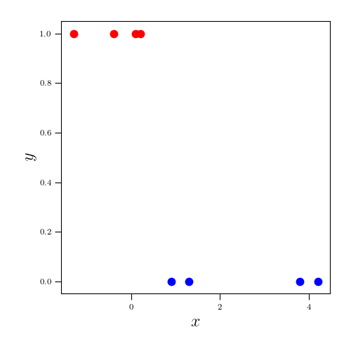
In this simple example, our goal in the first step of applying a CART model is to draw a vertical line such that the two classes of points are maximally segregated by this line. As we will explore in more detail below, there are several ways to quantitatively measure the quality of this segregation of points.
For binary outcomes, one of the most popular ways is to find splits that minimize the overall entropy of the bins. Recall that the entropy for a binary random variable $z$ with $p(z = 1) = \rho$ is given by
\[H(z) = -\rho \log \rho.\]Within a given region $R \subseteq \mathcal{X}$ of the predictor space, suppose $\rho_0 \in [0, 1]$ is the fraction of the samples with label $y=0$, and $\rho_1$ is the fraction of the samples with label $y=1$. Then we define the entropy within this region as a sum:
\[H(R) = -\rho_0 \log \rho_0 -\rho_1 \log \rho_1.\]For this example, let’s denote the subsets of the predictor space below and above a given threshold as $\mathcal{X}^\tau_L = \{x \in \mathcal{X}: x \leq \tau\}$ and $\mathcal{X}^\tau_R = \{x \in \mathcal{X}: x > \tau\}$. We then compute the entropy induced by a given threshold $\tau$ as the weighted average of the entropy of the data on each side of the split (where the weights are the fraction of data samples in each region):
\[E_\tau = \frac{|X^\tau_L|}{n} H(\mathcal{X}^\tau_L) + \frac{|X^\tau_R|}{n} H(\mathcal{X}^\tau_R)\]where $|X^\tau_L|$ and $|X^\tau_R|$ are the number of samples on the left and right of $\tau$, respectively.
Consider the animation below, where we consider a number of different thresholds $\tau$ (as indicated by the moving vertical line in the left panel). In the right panel, we show the entropy induced by splitting the points at a given value (the current entropy shown with a red dot).
In this case, a perfect split of the data exists, under which the split achieves an entropy of $0$. Of course, this is highly unlikely to happen in practice, but demonstrates what a good split looks like for this toy example.
In this case, we only required one split of the predictor space to achieve perfect performance on the training data. If this weren’t the case, then we would continue to recursively partition the input space. These two-way splits of the data space can be represented as a binary tree, where each node represents one of the partitions. The terminal nodes then contain the subsets of the predictor space with similar response values. This is the basic idea behind fitting CART models, as we’ll explore in more depth below.
Now that we have an intuitive sense of our goal, let’s turn to a more formal algorithm for fitting these trees.
The basic algorithm
As we saw above, the central idea behind CART models is to recursively find partitions of the dataset, which results in a tree of binary decisions. When the tree is formed, each of these decisions is of the form,
“Does feature $j$ in sample $i$ belong to $\mathcal{X}_L$ or $\mathcal{X}_R$?”
Here $\mathcal{X}_L$ and $\mathcal{X}_R$ are two disjoint sets (corresponding to “left child” and “right child” of a given node in the tree) where $\mathcal{X}_L \cup \mathcal{X}_R = \mathcal{X}$, $\mathcal{X}_L \cap \mathcal{X}_R = \emptyset$, and $\mathcal{X}$ is the predictor space.
The goal when fitting CART models is then to define the sets $\mathcal{X}_L$ and $\mathcal{X}_R$ at each level of the tree such that our predictive model achieves the best performance possible. In most cases, choosing these sets at each level of the tree will be equivalent to finding a threshold $\tau$ that partitions the predictor space such that $\mathcal{X}_L = \{\mathbf{x} : x^j \leq \tau \}$ and $\mathcal{X}_R = \{\mathbf{x} : x^j > \tau \}$, where $x^j$ is the $j$th feature of $\mathbf{x}$.
To identify the best possible split, we need a way to compare the quality of any two splits. This is typically done by computing a measure of “impurity” of the resulting splits. Intuitively, we can think of the impurity as the amount of mixing between samples with dissimilar response variables in each node. In fitting CART models, we seek to minimize the impurity. Conversely, we want to maximize the “purity” of each node so that samples with similar response values end up in the same terminal node of the tree.
Putting these steps together into an algorithm, we have the following algorithm sketch:
- Begin at the root node of the tree (containing the full dataset $\{(\mathbf{x}_i, y_i)\}_{i=1}^n$).
- Until convergence:
- Compute the impurity induced by every possible partition of the data, where each partition is defined by a threshold $\tau$.
- Identify the threshold $\tau^\star$ with minimal impurity and create two children containing these subsets.
- Recurse on the children $(x_i, y_i)_{\leq \tau^\star}$ and $(x_i, y_i)_{> \tau^\star}$.
To make predictions for a test sample $\mathbf{x}^\star$, we then follow through the decisions in the tree. At the leaf node, we typically predict $\widehat{y}^\star$ to be the majority class in this terminal node (in the classification setting) or the average value in this terminal node (in the regression setting).
Let’s return to our one-dimensional example to demonstrate how CART fitting works. Below is an animation that recursively finds the best split of the data (shown by the vertical lines). It exhaustively loops over every possible split and computes the entropy of each, as shown by the moving black line on the left. Once an optimal split is found, we fix that partition (shown in a gray line) and recurse on the remaining branches that still have mixed classes.
Implementing CART models in Python
CART models are relatively simple to implement. Not surprisingly, we rely on a binary tree data structure to encode the splits in the data. Below, we show a demonstrative implementation for one-dimensional inputs.
We rely on two Python classes: CART and Node. The CART class implements a binary tree with a function split that finds the current optimal split for a set of data. The Node class contains one node in the tree and its associated data.
import numpy as np
from scipy.stats import entropy

class CART:
  def __init__(self):
    pass

  def fit(self, X, Y):
    self.root = Node(X, Y)
    self.split(self.root)

  def split(self, node):

    # Stop if all samples belong to same class
    # (this includes the case when there's only one sample at this node)
    if len(np.unique(node.Y)) == 1:
      node.split = "Terminal"
      return

    best_split = self.find_best_split(node.X, node.Y)

    # Create children nodes
    left_idx = np.where(node.X <= best_split)[0]
    right_idx = np.where(node.X > best_split)[0]
    X_left, Y_left = node.X[left_idx], node.Y[left_idx]
    X_right, Y_right = node.X[right_idx], node.Y[right_idx]
    node.left_child = Node(X_left, Y_left)
    node.right_child = Node(X_right, Y_right)
    node.split = best_split

    # Recurse on left and right nodes
    self.split(node.left_child)
    self.split(node.right_child)

  def find_best_split(self, X, Y):
    # Find best split
    n = X.shape[0]
    split_candidates = np.zeros(n - 1)
    for ii in range(n - 1):
      split_candidates[ii] = X[ii:ii+2].mean()

    # Compute entropies
    entropies = np.zeros(len(split_candidates))
    for ii in range(len(split_candidates)):
      curr_left_bin_idx = np.where(X <= split_candidates[ii])[0]
      curr_right_bin_idx = np.setdiff1d(np.arange(n), curr_left_bin_idx)

      frac1s_left = (Y[curr_left_bin_idx] == 1).sum() / curr_left_bin_idx.shape[0]
      frac0s_left = (Y[curr_left_bin_idx] == 0).sum() / curr_left_bin_idx.shape[0]
      frac1s_right = (Y[curr_right_bin_idx] == 1).sum() / curr_right_bin_idx.shape[0]
      frac0s_right = (Y[curr_right_bin_idx] == 0).sum() / curr_right_bin_idx.shape[0]

      entropy_left = entropy(pk=[frac1s_left, frac0s_left])
      entropy_right = entropy(pk=[frac1s_right, frac0s_right])

      # Weighted avg
      curr_entropy = len(curr_left_bin_idx) / n * entropy_left + len(curr_right_bin_idx) / n * entropy_right
      entropies[ii] = curr_entropy

    best_split = split_candidates[np.argmin(entropies)]
    return best_split

class Node:
  def __init__(self, X, Y):
    self.X = X
    self.Y = Y
    self.left_child = None
    self.right_child = None
    self.split = None
We can fit this code on our previous example. Thanks to the printing function from this StackOverflow answer, we can also visualize the resulting tree:
     ___-2.0__________
    /                 \
Terminal         ___-0.5__________
                /                 \
            Terminal         ___1.22____
                            /           \
                        Terminal    Terminal
In this diagram, each node is either shown by a number (the threshold for each split) or the word “Terminal” (in which case this is a leaf node).
Time complexity
An important consideration for CART models is the time complexity of the fitting procedure.
When the predictors are continuous, there are $p (n - 1)$ possible splits of the data, where $n$ is the number of samples and $p$ is the number of features. Recall that we can sort a list of length $n$ in time $O(n \log n)$. Doing this for each of the $p$ features then extends the time complexity to $O(p n \log n)$.
When the predictors are categorical with $k$ unique classes, there are $2^{k-1} - 1$ possible partitions. In the full CART fitting algorithm, we must loop over all of these.
Thus, fitting these models can be computationally demanding when the number of samples or number of classes is large. Some more recent work has developed faster methods that use approximations to find partitions that are close to optimal.
Pruning
If we run the above algorithm exhaustively, we will eventually terminate the training procedure when each training sample belongs to its own partition/terminal node. However, allowing the tree to achieve this level of granularity in the predictor space can result in overfitting. Given a held-out test sample, if we were to predict with this overfit tree, it may be overly influenced by the particular training set.
More technically, this is an instance if a bias-variance tradeoff. As we allow the tree to become more complex, we obtain lower error (bias) on the training set, but we also run the risk of overfitting to any given training set (variance).
One common way to combat the issue of overfitting in CART models is to perform a post-hoc “pruning” process in which leaves of the tree are removed. Removing leaves of the tree is effectively equivalent to re-combining parts of the predictor space that had been partitioned in the fitting process. A popular way of deciding which leaves to prune is to use a “validation” set of data samples, and iteratively remove leaf nodes, which will typically result in a decrease in the validation error. This process can be repeated until the validation error begins to increase again.
Connection to logistic regression
For the linear model-minded crowd, an interesting connection is to view the partition at each CART node as a particular instance of logistic regression.
Recall that, for binary outcomes, logistic regression uses a linear transformation of the predictors to optimally split the two classes of responses. Specifically, a logistic regression model tries to find a coefficient vector $\boldsymbol{\beta} \in \mathbb{R}^p$ and an intercept $\beta_0$. The linear predictor is then given by $\mathbf{x}^\top \boldsymbol{\beta}$, which can then be transformed to be in the range $(0, 1)$. This transformation is usually chosen to be the logistic function:
\[p_i = \frac{1}{1 + \exp(-\mathbf{x}^\top \boldsymbol{\beta} + \beta_0)}.\]Intuitively, the coefficients $\boldsymbol{\beta}$ control how “steep” the logistic function is when discriminating between two classes. For instance, the animation below shows the logistic function for a range of values for $\boldsymbol{\beta}$ in a one-dimensional example. Typically classification is performed such that class $1$ is predicted when $p_i > 0.5.$
As we can see, the curve becomes steeper and steeper for larger absolute values of the coefficient $\beta$. When $\beta \in \{-\infty, \infty\}$, we obtain a perfect step function.
On the other hand, the intercept $\beta_0$ controls the overall location of this logistic curve. In the animation below, we can see that the curve is translated left or right depending on the value of $\beta_0$.
Thus, to frame CART models in terms of logistic regression, at each node, CART models are essentially fitting the intercept of a logistic regression model where the coefficient vector is fixed at $\infty$ or $-\infty$ (depending on which class is in which partition).
References
- Breiman, Leo, et al. “Classification and regressiontrees, wadsworth statistics.” Probability Series, Belmont, California: Wadsworth (1984).
- Mihaela van der Schaar’s notes on CART models
- Loh, Wei‐Yin. “Classification and regression trees.” Wiley interdisciplinary reviews: data mining and knowledge discovery 1.1 (2011): 14-23.