Andy Jones
Bayesian optimal experimental design
\(\DeclareMathOperator*{\argmin}{arg\,min}\) \(\DeclareMathOperator*{\argmax}{arg\,max}\)
Performing experiments in the natural and social sciences can be costly in terms of both time and money. Thus, there’s an incentive to design experimental setups so that the experiments are maximally informative and their cost is minimized.
In this post, we explore principled ways to choose experimental designs using Bayesian inference. These approaches – which are generally called “Bayesian optimal experimental design” (BOED) – use model-based inference to choose a design that is most likely to be “useful” to the experimenter.
Here, we’ll walk through an example of performing BOED, describing the methodological details as we go. This example is inspired by the Pyro example on BOED.
Identifying spice tolerance
Suppose want to determine a person’s tolerance of spicy foods. To do so, we can feed them a sequence of peppers, each with a known score on the Scoville Scale, and have the person say whether this is too spicy for their preference or not.
To formalize this problem, denote pepper $t$’s Scoville score as $x_t \in \mathbb{R}_+$, and let $y_t \in \{0, 1\}$ be the person’s decision about the $t$th pepper, where $0$ represents “tolerable” and $1$ represents “intolerable.” We assume the person has a true tolerance $\theta$ (which is unknown to the experimenter) such that they tolerate all peppers with Scoville score less than $\theta$.
Let’s model this person’s spice tolerance using a logistic regression model that contains just an intercept term. Consider the following model:
\[y \sim \text{Bern}(g(\theta)),~~g(\theta) = \frac{1}{1 + e^{-\theta}},~~\theta \sim \mathcal{N}(\mu_0, \sigma^2_0).\]Here, $\theta$ represents a threshold for spice tolerance. Although the Scoville score must be nonnegative, we model $\theta$ with a Gaussian defined on $\mathbb{R}$ for simplicity.
In a classical Bayesian approach to inference, given a dataset $\{(x_t, y_t)\}_{t=1}^T$ of $T$ responses, we would like to perform inference on $\theta$ by computing the posterior:
\[p(\theta | \mathbf{y}_{1:T}, \mathbf{x}_{1:T}),\]where $\mathbf{y}_{1:T} = (y_1, \cdots, y_T)^\top$ and $\mathbf{x}_{1:T} = (x_1, \cdots, x_T)^\top$. However, how these $T$ trials were designed could greatly affect the accuracy and precision of the inferences we make about $\theta$. Choosing these $T$ peppers optimally is the business of experimental design, as we’ll see next.
Optimizing experimental design
There are several ways we could perform this experiment. Suppose we limit ourselves to testing $T < \infty$ peppers, and suppose we only have an finite set of peppers $\mathcal{P}$ available to us that we can choose from. Here are a few ways we could choose them:
- We could choose $T$ peppers at random.
- We could choose $T$ peppers with linearly spaced Scoville scores.
- We could choose $T$ peppers with logarithmically spaced Scoville scores.
- Or, as we explore in this post, we could adaptively choose each pepper based on our observations so far.
To adaptively adjust our experimental design, we’ll choose $x_t$ by leveraging the existing data $\{(x_i, y_i)\}_{i=1}^{t-1}$. To do so, we need to define the “utility” of a given experiment, which roughly measures how good the experiment and its outcome are for our purposes.
More formally, a utility function $\mathcal{U}$ maps from the design space $\mathcal{X}$, the parameter space $\Theta$, and the outcome space $\mathcal{Y}$ to a number (which is typically nonnegative) representing how “helpful” or “good” an experiment is:
\[\mathcal{U} : \mathcal{X} \times \Theta \times \mathcal{Y} \mapsto \mathbb{R}_+.\]When our central goal is to perform inference on a model parameter (as is the case with our spice tolerance experiment), a common choice of utility function is the information gain (IG). IG measures the reduction in the entropy in the posterior before and after performing an experiment with design $x_t$:
\[\text{IG}(x_t) = \underbrace{H\left[ p(\theta | \mathbf{y}_{1:t-1}) \right]}_{\text{Entropy before experiment}} - \underbrace{H\left[ p(\theta | \mathbf{y}_{1:t}, x_t) \right]}_{\text{Entropy after experiment}},\]where $H\left[ p(a) \right] = -\int_\mathcal{A} p(a) \log p(a) da$ is the entropy of a distribution $p(a)$.
In many cases when all of the terms are fully observed, we can compute these entropy terms (or at least estimate them). However, in the setting of experimental design, we don’t know the outcome of the experiment $y_t$ before running it, which means we also can’t compute the posterior for $\theta$. Instead, we can take the expected value of the IG (often called the EIG) over $y_t$:
\begin{equation} \text{EIG}(x_t) = \mathbb{E}_{y_t}\left[H\left[ p(\theta | \mathbf{y}_{1:t-1}) \right] - H\left[ p(\theta | \mathbf{y}_{1:t}) \right] \right]. \end{equation}
Intuitively, we can understand the EIG of a design $x_t$ as the amount of information (in the Shannon sense) we expect to hypothetically obtain about $\theta$ after running this experiment and observing $y_t$.
We can rearrange this expression (see Appendix) into a more convenient form:
\begin{equation} \text{EIG}(x_t) = \mathbb{E}_{\theta, y_t}\left[\log \frac{p(\mathbf{y}_t | \theta)}{p(\mathbf{y}_t)} \right]. \label{eq:eig} \tag{1} \end{equation}
Finding the maximizer of the EIG then gives us a method for sequentially choosing experimental designs. On iteration $t$, our policy will be to choose the design $x_t^\star$ that maximizes the expected information gain:
\[x_t^\star = \argmax_{x \in \mathcal{X}} \text{EIG}(x).\]Nested Monte Carlo approximation
Equation \ref{eq:eig} contains an intractable double integral, so we need to find a way to approximate it. There have been several methods proposed (see References), but here we’ll focus on what is perhaps the most straightforward way to do this.
Here, we’ll use a simple Monte Carlo (MC) approach that approximates each integral with a finite sum. Because of the double integral, this is often called nested Monte Carlo (NMC). The basic approximation is as follows:
\[\frac{1}{N} \sum\limits_{n=1}^N \log \frac{p(y_n | \theta_{n, 0})}{\frac{1}{M} \sum\limits_{m=1}^M p(y_n | \theta_{n, m})},~~~\theta_{n, \star} \sim p(\theta | \mathbf{y}_{1:t-1}),~~~y_n \sim p(y_n | \theta_{n, 0}).\]Here $N$ is the number of MC samples for the outer sum, and $M$ is the number of samples for the inner sum. Note that, after the first iteration of experimentation, we will need to compute the posterior $p(\theta | \mathbf{y}_{1:t-1})$ in order to sample from it.
Example
Let’s now simulate an adaptive spice tolerance experiment using the tools we just developed. Let’s assume the person’s true spice tolerance is $\theta^\star = 20,000$ on the Scoville scale. Of course, we don’t know this value when running the experiment, but we’ll use it to simulate the outcome of each experiment.
Suppose we have a set of $20$ peppers with evenly spaced Scoville scores $x \in \{6, 7, 8, \cdots, 25\}$. However, due to time constraints, we can only run $10$ rounds of the experiment, where we select one pepper to feed the subject on each round. We are allowed to re-select the same pepper on multiple rounds. How should we choose the sequence of peppers?
Let’s assume our prior is slightly biased, and we underestimate the person’s spice tolerace, although we have fairly high uncertainty. We’ll encode this in our prior as:
\[\theta \sim \mathcal{N}(15, 8).\]On the first step of experimentation, we don’t have any data yet. Thus, when we compute the EIG, we’ll use the prior distribution $p(\theta)$ as a baseline rather than the running posterior. We can compute the EIG for every pepper, which we plot below in black, along with the prior distribution for $\theta$ in red.
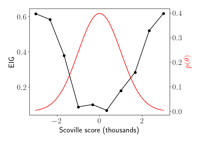
We’ll select the pepper with the highest EIG, which in this case is $x_1^\star = 15$, the same as the mean of our prior for $\theta$. We run this experiment and observe that the person response $0$, or that they can tolerate this pepper.
Now, we can repeat this EIG calculation, but this time we can use our observation to influence our next design. Below, we show an animation of the EIG (black curve) and updated posterior (red curve) across rounds of the experiment.
Notice how the selected pepper tends to approach the true tolerance $\theta^\star = 20$ quickly, and then explores the local region around this value. This adaptive design ultimately sharpens our posterior around the true value, resulting in less uncertainty about our inference for $\theta$.
By contrast, we can also simulate an experiment in which we naively choose $10$ peppers that are evenly spaced on the Scoville scale, $x \in \{ 6, 8, 10, \cdots, 24 \}$. We can then compare the final posterior learned from this experiment to the final posterior learned from our adaptive experiment.
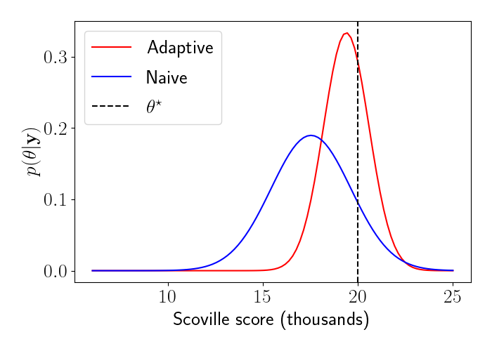
We observe that the adaptive design ultimately allows for more precise inference about $\theta$ compared to a naive experimental design.
Appendix
We can rearrange the expression for EIG as follows:
\begin{align} \text{EIG}(x_t) &= \mathbb{E}_{\theta, y_t}\left[H\left[ p(\theta | \mathbf{y}_{1:t-1}) \right] - H\left[ p(\theta | \mathbf{y}_{1:t}) \right] \right] \\ &= \mathbb{E}_{\theta, y_t}\left[-\mathbb{E}_{p(\theta | \mathbf{y}_{1:t-1})} \left[ \log \frac{p(\mathbf{y}_{1:t-1} | \theta) p(\theta)}{p(\mathbf{y}_{1:t-1})} \right] + \mathbb{E}_{p(\theta | \mathbf{y}_{1:t})} \left[ \log \frac{p(\mathbf{y}_{1:t} | \theta) p(\theta)}{p(\mathbf{y}_{1:t})} \right] \right] \\ &= \mathbb{E}_{\theta, y_t}\left[-\mathbb{E}_{p(\theta | \mathbf{y}_{1:t-1})} \left[ \log \frac{p(\mathbf{y}_{1:t-1} | \theta) p(\theta)}{p(\mathbf{y}_{1:t-1})} \right] + \mathbb{E}_{p(\theta | \mathbf{y}_{1:t-1})} \left[ \log \frac{p(\mathbf{y}_{1:t-1} | \theta) p(\theta)}{p(\mathbf{y}_{1:t-1})} \right] + \mathbb{E}_{p(\theta | \mathbf{y}_{t})} \left[ \log \frac{p(\mathbf{y}_{t} | \theta)}{p(\mathbf{y}_{t})} \right] \right] \\ &= \mathbb{E}_{\theta, y_t}\left[\log \frac{p(\mathbf{y}_t | \theta)}{p(\mathbf{y}_t)} \right]. \end{align}
References
- Pyro example on BOED
- Foster, Adam, et al. “Variational Bayesian optimal experimental design.” Advances in Neural Information Processing Systems 32 (2019).
- Rainforth, Tom, et al. “On nesting monte carlo estimators.” International Conference on Machine Learning. PMLR, 2018.