Approximating kernels with random projections

\(\DeclareMathOperator*{\argmin}{arg\,min}\) \(\DeclareMathOperator*{\argmax}{arg\,max}\)

Constructing and evaluating positive semidefinite kernel functions is a major challenge in statistics and machine learning. By leveraging Bochner’s theorem, we can approximate a kernel function by transforming samples from its spectral density.

Below, we show how this approximation works. First, we provide a short review of Bochner’s theorem, which is the essential building block for this approach.

Bochner’s theorem

First, let’s review Bochner’s theorem.

Theorem (Bochner). Every positive definite function is the Fourier transform of a positive finite Borel measure.

In the context of kernels, we have a very important corollary.

Corollary. For any shift invariant kernel, $k(x - y)$, there exists a probability density function $p(w)$ such that

\[k(x - y) = \int_{\mathbb{R}} e^{-iw (x - y)} p(w) dw.\]

Sampling to approximate kernels

Suppose we have a density $p(w)$ and we’d like to find the corresponding kernel function $k$. From Bochner’s theorem above, recall that we know the relationship bewteen the density and the kernel:

We can get an unbiased approximation of this integral by taking samples from $p$, computing the term in the integrand, and taking the sample average of these terms. In particular, suppose we draw $K$ samples independently from $p$:

Then let’s compute the integrand term for each of these samples independently, $e^{-iw_k (x - y)}$ and arrange them into a vector:

Now, we can take the inner product of these two vectors,

where $\phi(x)^*$ is the complex conjugate of $\phi(x)$.

We can see that the summand term looks very much like the integrand term in Bochner’s theorem. In fact, if we divide this sum by $K$, we get an unbiased estimate of the kernel function:

\begin{align} \mathbb{E}_{p(w)} \left[\frac1K \sum\limits_{k=1}^K e^{-iw_k (x - y)}\right] &= \mathbb{E}_{p(w)} \left[e^{-iw_1 (x - y)} \right] \\ &= \int_{\mathbb{R}} e^{-iw (x - y)} p(w) dw \\ &= k(x - y). \end{align}

The first equality comes from the fact that each of the terms in the sum will have the same expectation, so it reduces to taking the expectation of an arbitrary sample (here, represented by $w_1$). To fully complete the projection, we can account for the $\frac1K$ term inside of the projection itself by multiplying by $\frac{1}{\sqrt{K}}$ (because this will become $\frac1K$ after taking an inner product). This results in

We can further simplify this to eliminate the imaginary component. Consider again the term $e^{-iw(x - y)}$. Recall a trigonometric identity based off of Euler’s formula:

Applying Euler’s formula once more to the first term on the right-hand side, we have

\begin{align} e^{-iw(x - y)} &= \cos(w(x - y)) + i\sin(w(x - y)) - 2i \sin (w(x - y)) \\ &= \cos(w(x - y)) - i\sin(w(x - y)). \end{align}

Since sine is an odd function, i.e. $\sin(-x) = \sin(x)$, we can see that an expectation of the $\sin$ term with respect to $p(w)$ will be zero. More generally, for any function $f(w)$, we have

\begin{align} \mathbb{E}_{p(w)}[\sin (f(w))] &= \int_{-\infty}^0 \sin (f(w)) p(w) dw + \int_{0}^\infty \sin (f(w)) p(w) dw \\ &= \int_{-\infty}^0 \sin (f(w)) p(w) dw - \int_{-\infty}^0 \sin (f(w)) p(w) dw \\ &= 0. \end{align}

Thus, for our purposes, we can ignore the imaginary part of the expression. Using yet another trig identity, we have

This final form implies that our final projection will be

Note, then, that the inner product between two randomly projected points $x$ and $y$ will be

Example

Consider a simple example. Let $p(w) = \mathcal{N}(0, 1)$, and let’s assume we have just two fixed inputs, $x = 1, y = 2$. We know that the true kernel associated with the density $p$ in this case is the exponentiated quadratic:

Using the procedure derived above, we can approximate this kernel function as follows.

1. Draw $K$ samples from $p$, $w_1, \dots, w_K \sim p(w)$.
2. Compute $\psi(x)^\top \psi(y)$.

Since we know the true value of the kernel, we can compare our approximation with the truth. Below, we plot our approximation error as a function of $K$, the total number of samples.

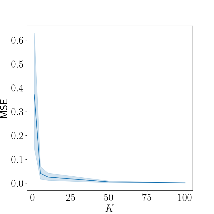
Clearly as $K$ increases, our approximation improves drastically. When $K \geq 50$, the error is nearly nonexistent.

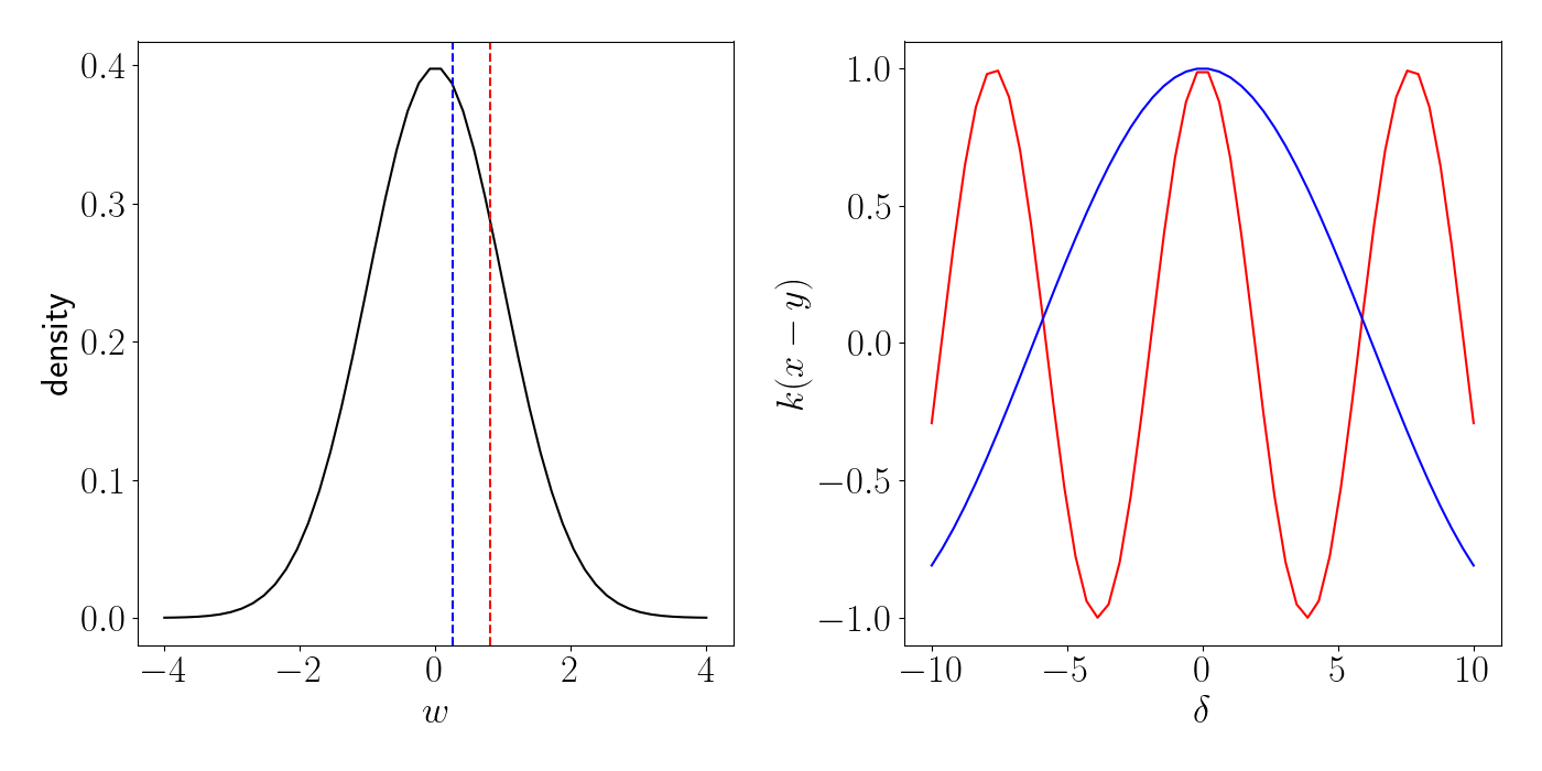
Let’s take another step into the details of how this approximation is working. For each sample from $p$, we get an unbiased estimate of the kernel function given by

The right side of this equality implies that the sample value $w_k$ controls the frequency of the resulting cosine wave. We can see this visually below. We draw two samples (one in red and one in blue) from $p$ on the left, and plot the resulting kernel function for each individually on the right.

Then, as we draw more samples (i.e., as we let $K$ increase), this amounts to drawing multiple of these waves and taking their average. The animation below illustrates this. We start out with just one sample, and then we incrementally increase $K$ one by one, keeping track of a running average on the right panel. As $K$ increases, we see that the function on the right approaches the exponentiated quadratic.

Code

Below is the code to produce the animation.

import numpy as np
import matplotlib.pyplot as plt
from scipy.stats import norm
from sklearn.gaussian_process.kernels import RBF
import matplotlib.animation as animation
import matplotlib.image as mpimg
import os

from os.path import join as pjoin

import matplotlib
font = {"size": 25}
matplotlib.rc("font", **font)
matplotlib.rcParams["text.usetex"] = True

SAVE_DIR = "/path/to/save"

xvalues = np.linspace(-10, 10, 50)
yvalues = np.linspace(-10, 10, 50)
xx, yy = np.meshgrid(xvalues, yvalues)
points = np.concatenate([np.atleast_2d(xx.ravel()), np.atleast_2d(yy.ravel())]).T
deltas = points[:, 0] - points[:, 1]

xs = np.linspace(-4, 4)
ys = norm.pdf(xs)
w_samples = np.random.normal(size=100)
amplitudes = np.zeros(len(points[:, 1]))

for ii, ww in enumerate(w_samples):
    plt.figure(figsize=(14, 7))
    plt.cla()
    plt.subplot(121)
    plt.plot(xs, ys, color="black")
    plt.xlabel("w")
    plt.ylabel("density")
    plt.axvline(ww, linestyle="--", color="red")
    amplitudes += np.cos(ww * (0 - points[:, 1]))

    plt.subplot(122)
    plt.plot(points[:, 1], amplitudes / (ii + 1), color="black")
    plt.xlabel(r"$\delta$")
    plt.tight_layout()
    plt.savefig(pjoin("tmp", "tmp{}.png".format(ii)))
    plt.close()


fig = plt.figure()
ims = []
for ii in range(len(w_samples)):
    fname = "./tmp/tmp{}.png".format(ii)
    img = mpimg.imread(fname)
    im = plt.imshow(img)
    ax = plt.gca()
    ax.set_yticks([])
    ax.set_xticks([])
    ims.append([im])
    os.remove(fname)


writervideo = animation.FFMpegWriter(fps=5)

ani.save(pjoin(SAVE_DIR, "bochner_animation.mp4"), writer=writervideo, dpi=1000)

References

• Greg Shakhnarovich’s notes on random projections
• Rahimi, Ali, and Benjamin Recht. “Random Features for Large-Scale Kernel Machines.” NIPS. Vol. 3. No. 4. 2007.
• Greg Gundersen’s post on random features.