Andy Jones
Binomial model for options pricing
The binomial model is a simple method for determining the prices of options.
Basic binomial model assumptions
The binomial model makes a few simplifying assumptions (here, we’ll assume the underlying asset is a stock):
- In a given time interval, a stock price can only make two types of moves: up or down. Furthermore, each of these moves is by a fixed amount.
- All time intervals are discretized.
While these assumptions are fairly unrealistic, the model can be a good starting point for understanding more complex models. The binomial model is a discrete-time approximation to other, more interesting models, so it’s a good place to start. (Note that below we sometimes drop the $ sign to avoid notational clutter.)
Starting example
Consider a call option $V$ for a stock $S$ that is currently worth $100. Recall that the earnings from a call option will be positive for increases in the underlying’s value, but will be 0 for a decrease in the underlying stock. The earnings from a call option can be visualized in the plot below:
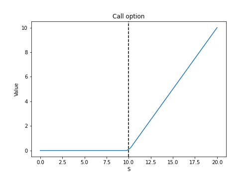
If the stock goes up by 1 tomorrow, the option is worth 1. If the stock goes down by 1 tomorrow, the option is worth 0.
The main question is: how much is the option worth today?
Without knowing anything else about the situation or the market, it seems like the answer will depend on the probability $p$ that the stock will go up (and equivalently the probability $1-p$ that it will go down). Indeed, the expected value of the option is \(\mathbb{E}[V] = px,\) where $x$ is the amount the stock could go up tomorrow. In this case $x=1$, so $\mathbb{E}[V] = p$.
However, due to the opportunity for investors to hedge their bets, this reasoning is faulty.
Consider the case when $p=0.2$, and the option costs $0.20$. Suppose an investor buys the call option $V$ and simultaneously takes a short position in $\frac12$ of the stock $S$, which costs $\frac12(100)=50$ in this case. Then this portfolio $P$ is worth \(P = \underbrace{0.2}_{\text{option}} - \underbrace{50}_{\text{short}}=-49.8.\) How much will the portfolio be worth tomorrow? There are two scenarios:
\begin{align} &\text{$S$ increases by 1} \implies P = 1-\frac12(101)=-49.50. \\ &\text{$S$ decreases by 1} \implies P = 0-\frac12(99)=-49.50. \end{align}
In either case, the portfolio will be worth $49.50$. If the investor were to buy back the short position tomorrow, he or she would have gained $0.30$ without assuming any risk at all. This is an arbitrage opportunity.
Alternatively, if the option costs $0.50$ initially, then the initial portfolio is worth $49.50$, and there is no opportunity for riskless profit.
Interest rates
In practice, there is another, simpler way to make a risk-free profit: through the risk-free interest rate (usually approximated by bonds). The return on these bonds is the interest rate. Thus, we should factor this opportunity into the calculation of the option price.
Denote the interest rate as $r$. (For simplicity, we’ll assume $r$ is the daily return.) If we currently own $50$ in cash, then by buying bonds, we could have a portfolio worth $50(1+r)$ tomorrow without assuming any risk. Thus, we should discount tomorrow’s portfolio value by $\frac{1}{1+r}$ to account for this.
In the example above, this would mean
\begin{align} &V - \frac12(100) = -49.5\left(\frac{1}{1+r}\right) \\ \implies& (1+r)(V-50) = -49.5 \\ \implies& V-50+rV-50r=-49.5 \\ \implies& V=\frac{0.5+50r}{1+r} \end{align}
As an example, consider when $r=10^{-3}$. Plugging into the above, this implies that $V=0.504945$. Intuitively it makes sense that the option should cost slightly more than the no-interest case because the projected portfolio value tomorrow, \(-49.5\left(\frac{1}{1+10^{-3}}\right) = -49.495,\) which is a gain of $0.005$.
By simply working with bonds, our portfolio value would have been: \(50(1+10^{-3}) = 50.005\) for an equal gain of $0.005$.
More general form
Suppose the current time is $t$ and we’re considering the price of an option that expires at the next time step $t + \delta t$. The current stock price is $S$. There are two scenarios for the next time step:
- The stock price rises to $uS$, and the option price rises to $V^+$, making the portfolio worth $V^+ - \Delta uS$.
- The stock price falls to $vS$, and the option price falls to $V^-$, making the portfolio worth $V^- - \Delta vS$.
To figure out how much of the stock to short (represented by $\Delta$ here), we must hedge so that these two possible portfolios have equal value. \begin{align} &V^+ - \Delta uS = V^- - \Delta vS \\ \implies& \Delta = \frac{V^+ - V^-}{uS - vS}. \end{align} We can think of this quantity as a discrete approximation to “Delta”, or the sensitivity of the option to the change in the underlying stock price, \(\frac{V^+ - V^-}{uS - vS} \to \frac{\partial V}{\partial S} ~~~\text{as}~~~ \delta t \to 0.\)
The portfolio’s value at $t+\delta t$ then has two equivalent forms: \begin{align} P_{t + \delta t} &= V^+ - u \frac{V^+ - V^-}{u - v} \\ P_{t + \delta t} &= V^- - v \frac{V^+ - V^-}{u - v}. \end{align} To account for nonzero interest rates, this portfolio value must also be equal to the amount that could be earned just through the risk-free interest rate. Recall that if the interest rate is $r$ and the current value of the portfolio is $P$, then the value of the portfolio that just earns based on the interest rate at $t + \delta t$ is \(P_{t + \delta t} = P + Pr\delta t = P(1 + r \delta t)\) where $P = V-\Delta S$ is the original value of the portfolio.
Setting this value equal to the portfolio under the option investment, we have \begin{align} &P(1 + r \delta t) = V^+ - u \frac{V^+ - V^-}{u - v} \\ \implies& (V-\Delta S) (1 + r \delta t) = V^+ - u \frac{V^+ - V^-}{u - v} \\ \implies& \left(V-\left(\frac{V^+ - V^-}{uS - vS}\right) S\right) (1 + r \delta t) = V^+ - u \frac{V^+ - V^-}{u - v} \\ \implies& V(1 + r \delta t) - \left(\frac{V^+ - V^-}{u - v}\right) (1 + r \delta t) = V^+ - u \frac{V^+ - V^-}{u - v} \\ \implies& V(1 + r \delta t) = \left(\frac{V^+ - V^-}{u - v}\right) (1 + r \delta t) + V^+ - u \frac{V^+ - V^-}{u - v} \\ \implies& V(1 + r \delta t) = \left(\frac{V^+ - V^-}{u - v}\right) (1 + r \delta t) + \frac{u V^+ - v V^+}{u-v} - \frac{uV^+ - uV^-}{u - v} \\ \implies& V(1 + r \delta t) = \left(\frac{V^+ - V^-}{u - v}\right) (1 + r \delta t) + \frac{uV^- - vV^+}{u - v} \\ \end{align}
Suppose we choose to model the stock’s behavior as a random walk, where \(S_{t+\delta t} \sim \mathcal{N}(S_t + \mu \delta t, \sigma^2 S_t^2 \delta t)\)
We can then choose
\begin{align} u &= 1 + \sigma \sqrt{\delta t} \\ v &= 1 - \sigma \sqrt{\delta t} \\ p &= \frac12 + \frac{\mu \sqrt{\delta t}}{2\sigma} \end{align}
Plugging these values into the equation for the option price, we have \begin{align} &V(1 + r \delta t) = \left(\frac{V^+ - V^-}{(1 + \sigma \sqrt{\delta t}) - (1 - \sigma \sqrt{\delta t})}\right) (1 + r \delta t) + \frac{(1 + \sigma \sqrt{\delta t})V^- - (1 - \sigma \sqrt{\delta t})V^+}{(1 + \sigma \sqrt{\delta t}) - (1 - \sigma \sqrt{\delta t})} \\ \implies& V(1 + r \delta t) = \left(\frac{V^+ - V^-}{2\sigma \sqrt{\delta t}}\right) (1 + r \delta t) + \frac{V^- + \sigma \sqrt{\delta t} V^- - V^+ + \sigma \sqrt{\delta t} V^+}{2\sigma \sqrt{\delta t}} \\ \implies& V(1 + r \delta t) = V^+\left( \frac{1}{2\sigma \sqrt{\delta t}} + \frac{r \sqrt{\delta t}}{2 \sigma} - \frac{1}{2 \sigma \sqrt{\delta t}} + \frac12 \right) + V^- \left( -\frac{1}{2\sigma \sqrt{\delta t}} - \frac{r\sqrt{\delta t}}{2\sigma} + \frac{1}{2\sigma \sqrt{\delta t}} + \frac12 \right) \\ \implies& V(1 + r \delta t) = V^+ \underbrace{\left( \frac{r \sqrt{\delta t}}{2 \sigma} + \frac12 \right)}_{p} + V^- \underbrace{\left( - \frac{r\sqrt{\delta t}}{2\sigma} + \frac12 \right)}_{1-p} \end{align} The quantities $p$ and $1-p$ labeled with brackets above can be seen as the “risk-neutral probabilities”. In simple terms, these are the “probabilities” under which, if the stock obeyed them, the portfolio would have equal value at step $t+\delta t$ regardless of the direction of movement.
References
- Wilmott, Paul. Paul Wilmott on quantitative finance. John Wiley & Sons, 2013.