Andy Jones
BFGS
BFGS is a second-order optimization method – a close relative of Newton’s method – that approximates the Hessian of the objective function.
Throughout this post, we let $f(x)$ be the objective function which we seek to minimize.
Newton’s method
Newton’s method is one of the most fundamental second-order methods in optimization. The key idea is to form a second-order approximation of $f(x)$ at the current point, find the minimum of this approximation, and repeat.
Specifically, suppose we’d like to minimize $f(x)$ starting at $x_0$. Let $x \in \mathbb{R}$ be one-dimensional for simplicity for now. If we take a linear Taylor expansion of $f^\prime(x)$, we have
\[f^\prime(x) \approx f^\prime(x_0) + f^{\prime\prime}(x_0)(x - x_0).\]Setting this equal to zero, we have \begin{align} &f^\prime(x_0) + f^{\prime\prime}(x_0) x - f^{\prime\prime}(x_0) x_0 = 0 \\ \implies& x^\star = x_0 - \frac{f^{\prime}(x_0)}{f^{\prime\prime}(x_0)} \end{align}
This update is known as Newton’s method.
If $x \in \mathbb{R}^p$ and $p>1$, Newton’s method requires the gradient and Hessian:
\[x^\star = x_0 - [\nabla^2 f(x_0)]^{-1} \nabla f(x_0).\]Note that the size of the Hessian is $p \times p$ in this case. For high-dimensional optimization problems, storing these matrices may become difficult. Furthermore, finding the inverse Hessian could be difficult or computationally expensive. Approximating the Hessian (or its inverse) can yield great computational boosts without much loss in accuracy. One method that uses such a trick is BFGS.
BFGS
Consider again the scenario in which we are minimizing $f(x)$ where $x \in \mathbb{R}^p$. We are iteratively updating $x_k, k = 1, \dots, T$ where $T$ is determined by some convergence criterion.
Suppose we use a quadratic approximation to $f$ at each iteration. Denote this approximation at step $k$ as $\hat{f}_k(x)$. Specifically,
\[\hat{f}_k = f(x_k) + [\nabla f(x_k)]^\top (x - x_k) + \frac12 (x - x_k)^\top [\nabla f(x_k)]^2 (x - x_k).\]Now, instead of directly computing the Hessian $[\nabla f(x_k)]^2$, let’s approximate it. Call this approximation $B_k$. Various choices for $B_k$ form a famliy of methods called “quasi-Newton methods”. Here, we review one of the most popular approximations, which leads to the Broyden–Fletcher–Goldfarb–Shanno (BFGS) algorithm.
The BFGS update rule is the same as Newton’s method, simply replacing the Hessian with its approximation:
\[x_{k+1} = x_k - B_k^{-1} \nabla f(x_k).\]Suppose we are currently on step $k$, and we have just generated the next iterate $x_k$. Our goal is now to find a good $B_{k+1}$.
BFGS constrains $B_{k+1}$ such that the gradients of $\hat{f}_{k+1}$ are equal to the true gradients of $f$ at the most recent two points: $x_k$ and $x_{k+1}$. Note that the gradient of $\hat{f}_{k+1}$ is
\[\nabla \hat{f}_{k+1} = \nabla f(x_{k+1}) + B_{k+1} (x - x_{k+1}).\]Plugging in $x_{k+1}$, we can immediately see that the second condition is met:
\[\nabla \hat{f}_{k+1} = \nabla f(x_{k+1}) + B_{k+1} (x_{k+1} - x_{k+1}) = \nabla f(x_{k+1}).\]For the first condition we have
\begin{align} &\nabla \hat{f}_{k+1} = \nabla f(x_{k+1}) + B_{k+1} (x_k - x_{k+1}) = \nabla f(x_k) \\ \implies& B_{k+1} (x_{k+1} - x_k) = \nabla f(x_{k+1}) - \nabla f(x_k) \end{align}
Denoting $s_k = x_{k+1} - x_k$ and $y_k = \nabla f(x_{k+1}) - \nabla f(x_k)$, this simplifies to
\[B_{k+1} s_k = y_k.\]To make $B_{k+1}$ positive definite, we must have that
\[s_k^\top B_{k+1} s_k = s_k^\top y_k > 0.\]While the closely-related DFP algorithm parameterizes the problem in terms of the approximate Hessian $B_k$, BFGS parameterizes it in terms of the inverse Hessian $H_k := B_k^{-1}$. The constraints then become:
\[H_{k+1} y_k = s_k \;\;\text{ and }\;\; H_{k+1} = H_{k+1}^\top.\]We further specify $H_{k+1}$ by making as close to $H_k$ as possible.
\[H_{k+1} = \text{arg}\min_H \|H - H_k\| \;\;\; \text{ s.t. } H = H^\top, \;\; Hy_k = s_k.\]The solution is then given by
\[H_{k+1} = (I - \frac{1}{y_k^\top s_k} s_k y_k^\top) H_k (I - \frac{1}{y_k^\top s_k} y_k s_k^\top) + \frac{1}{y_k^\top s_k} s_k s_k^\top.\]This is the BFGS update rule. There are a couple important properties to notice about it:
- The inverse Hessian at step $k+1$ depends on the inverse Hessian at step $k$. This is unlike the traditional Newton’s method, which computes the inverse Hessian “from scratch” at each iteration.
- The update only depends on the previous inverse Hessian and the vectors $s_k$ and $y_k$. Furthermore, we only have to perform matrix multiplications and outer products (no inverses), so this update will be $\mathcal{O}(p^2)$, where $p$ is the dimension of $x$.
Simple example
To further build intuition, notice that when $p=1$, this update reduces to
\[H_{k+1} = \frac{s_k}{y_k} = \frac{x_{k+1} - x_k}{f^\prime(x_{k+1}) - f^\prime(x_{k})} = \left[ \frac{f^\prime(x_{k+1}) - f^\prime(x_{k})}{x_{k+1} - x_k} \right]^{-1}.\]This is simply a linear approximation to the (reciprocal) second derivative.
Suppose $f(x) = x^4$ is our objective function. Further, suppose $x_k = 4$ and $x_{k+1} = 2$. Then we can visualize the BFGS method by seeing that the approximation to the second derivative will just be the slope of a linear interpolation between the values of $f^\prime(x)$ at these two points. In this case, the computation is extremely simple:
\[f^{\prime\prime}_{k+1} \approx \frac{f^\prime(4) - f^\prime(2)}{4 - 2}.\]Here’s a plot of how this looks:
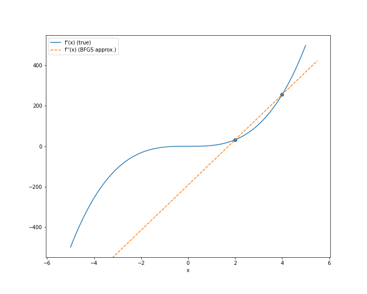
Notice that if $x_{k+1}$ and $x_k$ are extremely close to each other, the approximation will improve. In fact, in the limit, this reduces to the definition of a derivative:
\[f^{\prime\prime}(x) = \lim_{\epsilon \to 0} \frac{f^\prime(x + \epsilon) - f^\prime(x)}{\epsilon}.\]References
- Nocedal, Jorge, and Stephen Wright. Numerical optimization. Springer Science & Business Media, 2006.
- Wikipedia page on BFGS