Andy Jones
Belief propagation
Belief propagation is a family of message passing algorithms, often used for computing marginal distributions and maximum a posteriori (MAP) estimates of random variables that have a graph structure.
Computing marginals
Consider three binary random variables $x_1, x_2, x_3 \in {0, 1}$. Denote their joint distribution as $p(x_1, x_2, x_3)$. Suppose we want to compute the marginal distribution of $x_2$, $p(x_2)$. Naively, we can do this by summing over the other variables:
\[p(x_2) = \sum\limits_{x_1 \in \{0, 1\}} \sum\limits_{x_3 \in \{0, 1\}} p(x_1, x_2, x_3).\]This sum has 4 terms, one for each possible value of $(x_1, x_3)$. In general, finding the marginal of $x_i$ from the joint of $p$ total binary variables will require computing a sum with $2^{p-1}$ terms:
\[p(x_i) = \sum\limits_{x_1 \in \{0, 1\}} \cdots \sum\limits_{x_{i-1} \in \{0, 1\}} \sum\limits_{x_{i+1} \in \{0, 1\}} \cdots \sum\limits_{x_p \in \{0, 1\}} p(x_1, \dots, x_p).\]These sums become intractable for even moderate values of $p$, and also become intractable if the number of possible states of each variable is larger than two.
However, exploiting any special structure that exists between the variables can greatly expedite computing the marginals. Here, we explore the concept of factor graphs, and using these graphs to perform belief propagation with the goal of computing marginal distributions.
Factor graphs
Belief propagation is typically defined as operating on factor graphs. In their simplest form, factor graphs are a graph representation of a function of multiple variables. When a function factorizes in a certain way, factor graphs help represent the relationships between related variables.
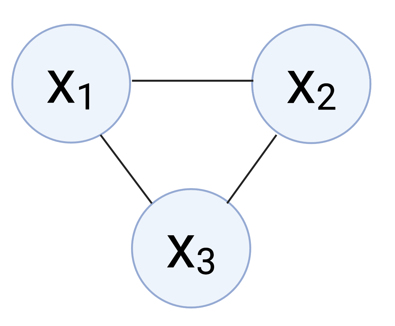
In the context of probability and statistics, factor graphs are usually used to represent probability distributions. For example, consider the joint distribution of three random variables $p(x_1, x_2, x_3)$. Without knowing anything else about their relationships, we can represent these variables in a fully-connected graph:
However, we may know more about the relationships between them. Suppose that $x_1$ and $x_3$ don’t directly depend on one another, and $x_3$ has its own special behavior. This means that the joint factorizes as
\[p(x_1, x_2, x_3) = p(x_1, x_2) p(x_2, x_3) p(x_3).\]We can think of this as having three “groups” of interrelated variables: one comprised of ${x_1, x_2}$, another comprised of ${x_2, x_3}$, and a third with just $x_3$. We can now represent these variables in the form of a factor graph. Factor graphs show the connections between the factors and the variables that those factors relate. In this case, we have the following graph:
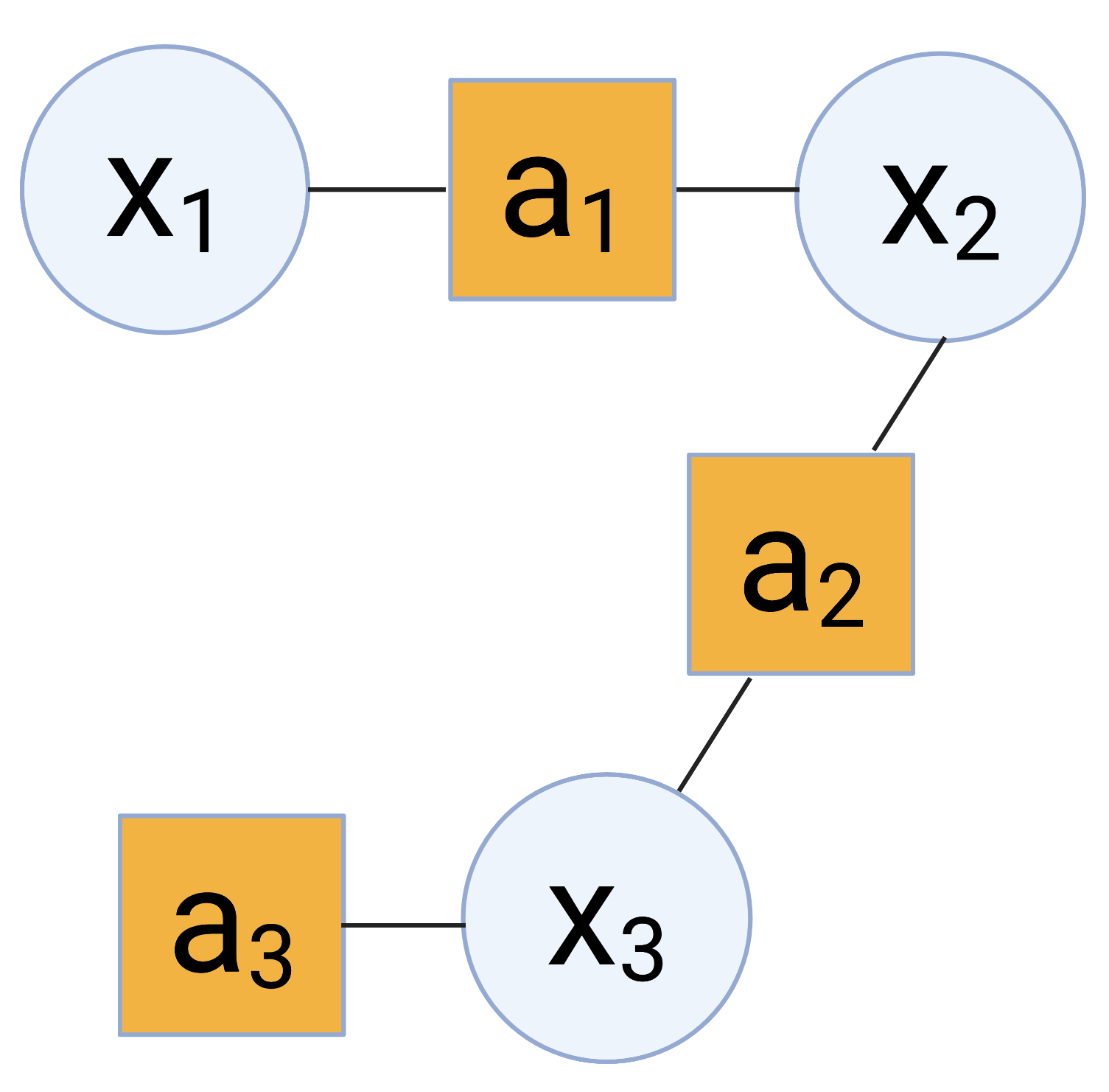
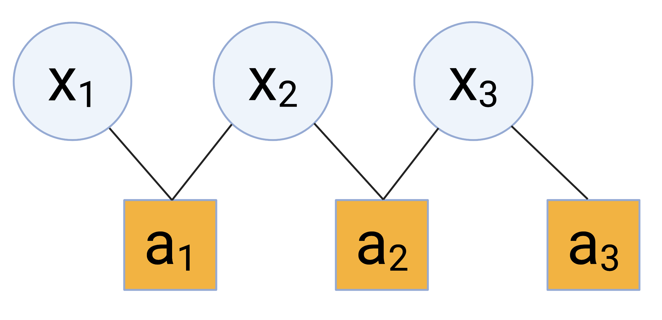
Factor graphs are always bipartite – we can shift the nodes in the above graph to show this clearly visually:
The “factors” in factor graphs help describe the relationships between the variable nodes, and help coordinate inference as we’ll see next.
Messages
As mentioned above, belief propagation is part of a family of algorithms known as “message-passing” algorithms. The name of this family means exactly what it sounds like: the nodes in the graph send “messages” to one another in order to learn about the overall structure of the variables.
In this post, we’ll denote a message from node $a$ to node $b$ as $\mu_{a \to b}$. In the context of probability and statistics, we can usually think about a message from $a$ to $b$ as node $a$ “encouraging” node $b$ to have some type of behavior. For example, in our example above, consider the message from $a_1$ to $x_2$, $\mu_{a_1 \to x_2}$. This message will encode what node $a_1$ “thinks” the state of $x_2$ should be based on its information about the relationship between $x_1$ and $x_2$.
The exact content of these messages – and how they’re passed – is dependent on the algorithm. Here, we’ll look at belief propagation’s protocol.
Belief propagation
Belief propagation updates the messages that are outgoing from a node based on the ones that are incoming to that node. This eventually spreads the information across the whole graph.
It’s an iterative algorithm that updates the messages at each timestep $t=1, \dots, T$. The algorithm is as follows. Note that in this post, we adopt the same notation as in the book Constraint Satisfaction networks in Physics and Computation, where $\partial a$ denotes the set of nodes immediately adjacent to $a$.
Belief propagation steps:
- $\mu_{j \to a}^{(t+1)}(x_j) = \prod\limits_{b \in \partial j \setminus a} \mu_{b \to j}^{(t)} (x_j)$
- $\mu_{a \to j}^{(t)} = \sum\limits_{\mathbf{x}_{\partial a \setminus j}} f_a(\mathbf{x}_{\partial a}) \prod\limits_{k \in \partial a \setminus j} \mu_{k \to a}^{(t)} (x_k).$
Belief propagation is also known as the “sum-product algorithm” because of the second step – in particular, the way that $\mu_{a \to j}$ is computed.
A useful outcome of belief propagation is that its messages can be used to estimate the marginal distributions of each variable. Specifically, the marginal for $x_i$ is estimated as the product of all incoming messages:
\[p(x_i) \propto \prod\limits_{a \in \partial x_i} \mu_{a \to x_i}^{(t-1)} (x_i).\]The product of these messages is only proportional to the marginal, so one must divide by the sum of the elements to make it sum to one.
Example
For example, consider the same example as in the sections above with variables $x_1, x_2, x_3$. Suppose we want to calculate the marginal distribution $p(x_2)$. Using the procedure above, we take the product of all messages incoming to $x_2$:
\[p(x_2 = \mathcal{X}_i) \propto \prod\limits_{a \in \partial x_2} \mu_{a \to x_2}[i]\]where $\mu[i]$ denotes the $i$th element of $\mu$.
Again, we’ll need to divide by the sum of the elements to make it sum to one.
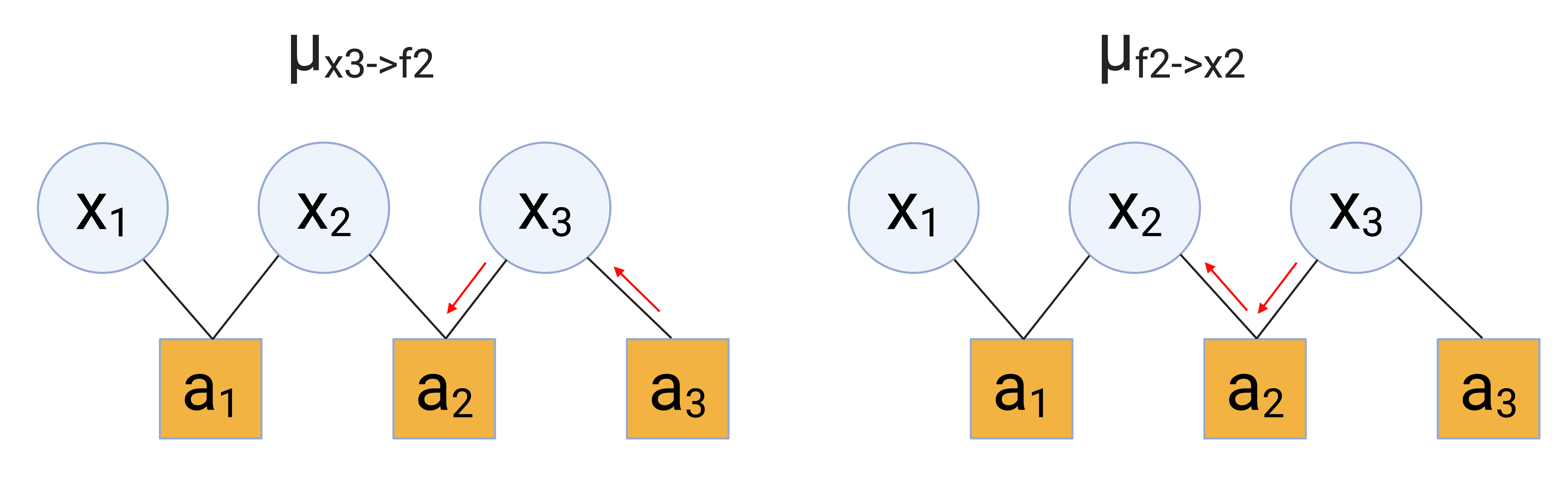
In this example, there are going to be two incoming messages to $x_2$: one from $a_1$ and one from $a_2$. To start, let’s compute the message going from $a_2$ to $x_2$, $\mu_{a_2 \to \mu_2}$. We have
\begin{align} \mu_{a_2 \to x_2} &= \sum\limits_{\mathbf{x}_{\partial a_2 \setminus x_2}} f_2(\mathbf{x}_{\partial a_2}) \prod\limits_{k \in \partial a_2 \setminus x_2} \mu_{k \to a_2} (x_k) \\ &= \sum\limits_{x_3 \in {0, 1}} f_2(x_3) \mu_{x_3 \to a_2} (x_3) \\ &= \sum\limits_{x_3 \in {0, 1}} f_2(x_3) \prod\limits_{b \in \partial x_3 \setminus a_2} \mu_{b \to x_3} (x_3) \\ &= \sum\limits_{x_3 \in {0, 1}} f_2(x_3) \mu_{f_3 \to x_3} (x_3). \\ \end{align}
Since $f_3$ doesn’t have any neighbors other than $x_3$, $\mu_{f_3 \to x_3} (x_3)$ reduces to $p(x_3)$. Continuing to simplify,
\begin{align} \mu_{a_2 \to x_2}[i] &= \sum\limits_{x_3 \in {0, 1}} p(x_2=i, x_3) 0.5 \\ &= p(x_2=i, x_3=0) p(x_3 = i) + p(x_2=i, x_3=1) p(x_3 = i). \\ \end{align}
Notice that to compute this update, we had to consider messages streaming all the way from $a_3$ to $x_2$. We can visualize these steps like so:
For the message coming from $a_1$, we have
\begin{align} \mu_{a_1 \to x_2} &= \sum\limits_{\mathbf{x}_{\partial a_1 \setminus x_2}} f_1(\mathbf{x}_{\partial a_1}) \prod\limits_{k \in \partial a_1 \setminus x_2} \mu_{k \to a_1} (x_k) \\ &= \sum\limits_{x_1 \in {0, 1}} f_1(x_1) \mu_{x_1 \to a_1} (x_1) \\ &= p(x_1 = 0, x_2 = i) 0.5 + p(x_1 = 1, x_2 = i) 0.5 \end{align}
Here, since $x_1$ doesn’t have any neighbors other than $a_1$, we assume that $\mu_{x_1 \to a_1} (x_1)$ is the uniform distribution over ${0, 1}$.
Putting these together, we obtain that the unnormalized marginal is
\begin{align} p(x_2=i) &\propto \underbrace{0.5 \left[p(x_1 = 0, x_2 = i) + p(x_1 = 1, x_2 = i) \right]}_{\text{Contribution from $\mu_{a_1 \to x_2}$}} \underbrace{p(x_3 = i) \left[ p(x_2=i, x_3=0)+ p(x_2=i, x_3=1) \right]}_{\text{Contribution from $\mu_{a_2 \to x_2}$}} \\ &= 0.5 \left[\sum\limits_{x_1} p(x_1, x_2=i)\right] \left[ \sum\limits_{x_3} p(x_2=i, x_3) p(x_3) \right]. \end{align}
In this case, we can see that belief propagation simply reduces to computing the marginal by “brute force”. In other words, since the joint distribution factorizes as
\[p(x_1, x_2, x_3) = p(x_1, x_2) p(x_2, x_3) p(x_3),\]this belief propagation equation is just the complete sum of the joint over $x_1$ and $x_3$. However, in more general situations, belief propagation will require iterative updating of the messages between nodes. I hope to provide a more complex example in a future post.
References
- Graph images were created with BioRender.com
- Constraint Satisfaction networks in Physics and Computation by Marc Mezard and Andrea Montanari.