Bayesian model averaging

Bayesian model averaging provides a way to combine information across statistical models and account for the uncertainty embedded in each.

Bayesian model averaging

Consider a set of $K$ statistical models $\mathcal{M}_1, \dots, \mathcal{M}_K$, each of which makes a different set of assumptions about the data generating process.

Typically, if we had just one model, we would often be interested in computing the posterior distribution of the parameters given the data $p(\theta | X)$. With multiple models, we can take a weighted average of the posterior under each model:

Here $p(\theta | \mathcal{M}_k)$ is the posterior of $\theta$ for just the one model $\mathcal{M}_k$, and $p(\mathcal{M}_k | X)$ is the “model probability”, or the probability of this model given the data.

The model probability can be expanded using Bayes’ rule:

\begin{align} p(\mathcal{M}_j | X) &= \frac{p(X | \mathcal{M}_j) p(\mathcal{M}_j)}{p(X)} \\ &= \frac{p(X | \mathcal{M}_j) p(\mathcal{M}_j)}{\sum\limits_{k=1}^K p(X | \mathcal{M}_k) p(\mathcal{M}_k) }. \\ \end{align}

Notice that this requires computing the marginal likelihood (or “evidence”) for each model $p(X | \mathcal{M}_k)$, which requires integrating out $\theta$:

Bayes factors

As a brief aside, another area where model probabilities and marginal probabilities must be computed is Bayes factors. Bayes factors are often used to compare the relative utility between two different models. Bayes factors arise as a part of the posterior odds between two models:

\begin{align} \frac{p(X | \mathcal{M}_1)}{p(X | \mathcal{M}_2)} &= \frac{\frac{p(\mathcal{M}_1 | X) p(X)}{p(\mathcal{M}_1)}}{\frac{p(\mathcal{M}_2 | X) p(X)}{p(\mathcal{M}_2)}} \\ &= \frac{p(\mathcal{M}_1 | X)}{p(\mathcal{M}_2 | X)} \cdot \frac{p(\mathcal{M}_2)}{p(\mathcal{M}_1)} \end{align}

When the models are given equal prior probabilities, $p(\mathcal{M}_1) = p(\mathcal{M}_2)$, this reduces to the ratio of model probabilities.

Beta-binomial example

Consider a set of coin tosses $X_1, \dots, X_n$, where $k$ of these flips turn up heads. Let $\sum\limits_{i = 1}^n X_i = Y$.

We can model the total number of heads $Y$ as

\begin{align} k &\sim \text{Binomial}(n, \theta) \\ \theta &\sim \text{Beta}(\alpha, \beta) \\ \end{align}

The posterior of $\theta$ is again a beta distribution:

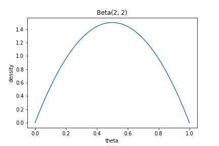
Consider two models. In the first model, we choose the parameters of the beta distribution so that most of the mass concentrates around $\theta = 0.5$:

\begin{align} k &\sim \text{Binomial}(n, \theta_1) \\ \theta_1 &\sim \text{Beta}(2, 2) \\ \end{align}

This prior has the shape in the plot below:

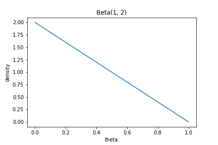
In the second model, we assume that the mass is more likely to lie in lower values of $\theta$:

\begin{align} k &\sim \text{Binomial}(n, \theta_2) \\ \theta_2 &\sim \text{Beta}(1, 2) \\ \end{align}

This prior has the shape in the plot below:

Now, how can we average these models to get a combined posterior for $\theta$?

We already computed the posteriors $p(\theta | \mathcal{M}_1, X)$ and $p(\theta | \mathcal{M}_2, X)$ above. Now, we must compute the model probabilities.

Starting with model 1, we have

\begin{align} p(\mathcal{M}_1 | X) &= \frac{p(X | \mathcal{M}_1) p(\mathcal{M}_1)}{\sum\limits_{k=1}^2 p(X | \mathcal{M}_k) p(\mathcal{M}_k) } \end{align}

This requires computing the marginal likelihood:

Luckily, in our simple beta-binomial model, this has a closed-form.

\begin{align} \int p(X | \theta, \mathcal{M}_1) p(\theta | \mathcal{M}_1) d\theta &= \int {n \choose k} \theta^k (1-\theta)^{n-k} \frac{\theta^{\alpha - 1} (1-\theta)^{\beta - 1}}{\text{Beta}(\alpha, \beta)} d\theta \\ &= {n \choose k} \frac{1}{\text{Beta}(\alpha, \beta)} \int \theta^{k + \alpha - 1} (1-\theta)^{n - k + \beta - 1} d\theta \\ &= {n \choose k} \frac{1}{\text{Beta}(\alpha, \beta)} \frac{\Gamma(k + \alpha) \Gamma(n - k + \beta)}{\Gamma(k + \alpha + n - k + \beta)} \\ &= {n \choose k} \frac{\text{Beta}(k + \alpha, n - k + \beta)}{\text{Beta}(\alpha, \beta)} \\ \end{align}

Plugging in the values for $\alpha$ and $\beta$ for each model and assuming $p(\mathcal{M}_1) = p(\mathcal{M}_2) = \frac12$,

\begin{align} p(\mathcal{M}_1 | X) &= \frac{{n \choose k} \frac{\text{Beta}(k + 2, n - k + 2)}{\text{Beta}(2, 2)} \cdot \frac12}{{n \choose k} \frac{\text{Beta}(k + 2, n - k + 2)}{\text{Beta}(2, 2)} \cdot \frac12 + {n \choose k} \frac{\text{Beta}(k + 1, n - k + 2)}{\text{Beta}(1, 2)} \cdot \frac12 } \\ &= \frac{\frac{\text{Beta}(k + 2, n - k + 2)}{\text{Beta}(2, 2)}}{ \frac{\text{Beta}(k + 2, n - k + 2)}{\text{Beta}(2, 2)} + \frac{\text{Beta}(k + 1, n - k + 2)}{\text{Beta}(1, 2)} } \\ \end{align}

Finally, the model-averaged posterior is

\begin{align} p(\theta | X) &= \frac{\theta^{2 + k - 1} (1-\theta)^{2 + n - k - 1}}{\text{Beta}(2, 2)} \frac{\frac{\text{Beta}(k + 2, n - k + 2)}{\text{Beta}(2, 2)}}{ \frac{\text{Beta}(k + 2, n - k + 2)}{\text{Beta}(2, 2)} + \frac{\text{Beta}(k + 1, n - k + 2)}{\text{Beta}(1, 2)} } \\ &+ \frac{\theta^{1 + k - 1} (1-\theta)^{2 + n - k - 1}}{\text{Beta}(1, 2)} \frac{\frac{\text{Beta}(k + 1, n - k + 2)}{\text{Beta}(1, 2)}}{ \frac{\text{Beta}(k + 2, n - k + 2)}{\text{Beta}(2, 2)} + \frac{\text{Beta}(k + 1, n - k + 2)}{\text{Beta}(1, 2)} } \\ \end{align}

Now, assume we observe 10 coin flips, 5 of which come up tails ($n=10, k=5$). If we plot the model-averaged posterior for these data, along with each individual model’s posterior, we can see that the averaged model has the effect that we would intuitively expect: it lies “in between” each of the two individual models.

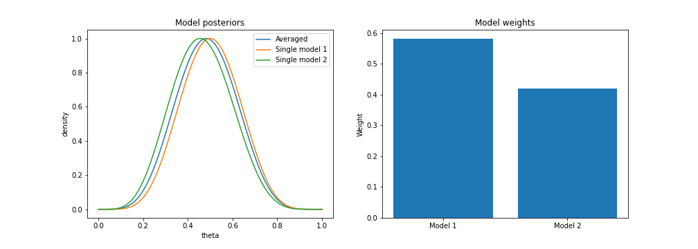
We also see that model 1 is given more weight, since it captures the data better.

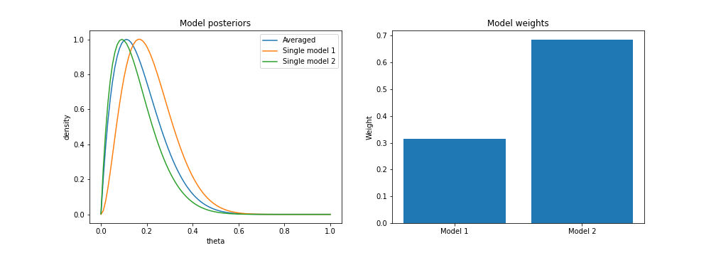
However, assume we only observe 1 tails flip out of 10. Then, we can see that model 2 is given more weight, but the averaged model still sits between the two individual models.

Below is the code to reproduce these plots:

import numpy as np
import matplotlib.pyplot as plt
from scipy.stats import beta as beta_distribution
from scipy.special import beta as beta_function

## Draw from Beta(1, 1)

alpha_param = 2
beta_param = 2
xs = np.linspace(1e-4, 1, 100)
ys = [beta_distribution.pdf(x, alpha_param, beta_param) for x in xs]

plt.plot(xs, ys)
plt.xlabel("theta")
plt.ylabel("density")
plt.title("Beta({}, {})".format(alpha_param, beta_param))
plt.show()

## Draw from Beta(2, 2)

alpha_param = 1
beta_param = 2
xs = np.linspace(1e-4, 1-1e-4, 100)
ys = [beta_distribution.pdf(x, alpha_param, beta_param) for x in xs]

plt.plot(xs, ys)
plt.xlabel("theta")
plt.ylabel("density")
plt.title("Beta({}, {})".format(alpha_param, beta_param))
plt.show()

## Compute model-averaged posterior

def posterior_pdf(theta, n, k, a1, b1, a2, b2):
    
    # Get weights for models
    first_model_weight = beta_function(k + a1, n - k + b1) / beta_function(a1, b1)
    second_model_weight = beta_function(k + a2, n - k + b2) / beta_function(a2, b2)
    total_model_weights = first_model_weight + second_model_weight
    
    model1_weight = first_model_weight / total_model_weights
    model2_weight = second_model_weight / total_model_weights
    
    # Get model pdfs
    model1_pdf = beta_distribution.pdf(theta, a1 + k, b1 + n - k)
    model2_pdf = beta_distribution.pdf(theta, a2 + k, b2 + n - k)
    
    total_density = model1_pdf * model1_weight + model2_pdf * model2_weight
    
    return total_density

def posterior_model_weights(n, k, a1, b1, a2, b2):
    
    # Get weights for models
    first_model_weight = beta_function(k + a1, n - k + b1) / beta_function(a1, b1)
    second_model_weight = beta_function(k + a2, n - k + b2) / beta_function(a2, b2)
    total_model_weights = first_model_weight + second_model_weight
    
    model1_weight = first_model_weight / total_model_weights
    model2_weight = second_model_weight / total_model_weights
    
    return model1_weight, model2_weight
    
## Compare to posterior of just one model

def beta_binomial_posterior(x, n, k, a, b):
    return beta_distribution.pdf(x, a + k, b + n - k)

n = 10
k = 1

plt.figure(figsize=(14, 5))

plt.subplot(121)

# Averaged posterior
a1, b1 = 2, 2
a2, b2 = 1, 2
xs = np.linspace(1e-4, 1-1e-4, 100)
ys = [posterior_pdf(x, n, k, a1, b1, a2, b2) for x in xs]
ys = ys / np.max(ys)
plt.plot(xs, ys, label="Averaged")

# Just one model's posterior
ys = [beta_binomial_posterior(x, n, k, a1, b1) for x in xs]
ys = ys / np.max(ys)
plt.plot(xs, ys, label="Single model 1")

ys = [beta_binomial_posterior(x, n, k, a2, b2) for x in xs]
ys = ys / np.max(ys)
plt.plot(xs, ys, label="Single model 2")

plt.xlabel("theta")
plt.ylabel("density")
plt.title("Model posteriors")
plt.legend()

plt.subplot(122)
m1_weight, m2_weight = posterior_model_weights(n, k, a1, b1, a2, b2)
plt.bar(np.arange(2), np.array([m1_weight, m2_weight]))
plt.xticks(ticks=np.arange(2), labels=["Model 1", "Model 2"])
plt.ylabel("Weight")
plt.title("Model weights")

plt.show()

References

• Hoeting, Jennifer A., et al. “Bayesian model averaging: a tutorial.” Statistical science (1999): 382-401.
• Bayesian model averaging: A systematic review and conceptual classification
• Gronau, Quentin F., et al. “A tutorial on bridge sampling.” Journal of mathematical psychology 81 (2017): 80-97.