Andy Jones
Autoregressive moving average models
\(\DeclareMathOperator*{\argmin}{arg\,min}\) \(\DeclareMathOperator*{\argmax}{arg\,max}\)
Setup
Suppose we’re modeling a sequence of univariate data $\{y_1, y_2, \dots\}$ where $y_t \in \mathbb{R}.$ For these types of data, we’re often interested in two broad objectives: forecasting future events and modeling historical behavaior of the sequence. Autoregressive and moving average models – as well as their combination – are useful and relatively simple models for these type of data. Below, we review each of these types of models in turn.
Autoregressive models
In an autoregressive model with lag $p,$ which we denote as $AR(p),$ the $t$th observation depends directly on the previous $p$ observations. The model is given by
\[y_t = \epsilon_t + \sum\limits_{i=1}^p \beta_i y_{t - i},~~~\epsilon_t \sim \mathcal{N}(0, \sigma^2)\]where $\{\beta_i\}$ are the coefficients, and $\sigma^2$ is the noise variance. Notice that $y_{t-1}$ depends on $y_{t - 2},$ $y_{t-2}$ depends on $y_{t-3},$ and so on. Thus, we can recursively unravel the model for $y_t$ back to the first observation $y_1.$
As an example of this, consider the $AR(1)$ model. We can expand $y_t$ as follows:
\begin{align} y_t &= \epsilon_t + \beta y_{t - 1} \\ &= \epsilon_t + \beta (\epsilon_{t-1} + \beta y_{t - 2}) \\ &= \epsilon_t + \beta (\epsilon_{t-1} + \beta (\epsilon_{t-2} + \beta y_{t-3})) \\ &\vdots \\ &= \beta^{t-1} y_1 + \sum\limits_{i=0}^{t-2} \beta^i \epsilon_{t - i}. \tag{1} \label{eq:ar1} \end{align}
This allows us to write the distribution of $y_t$ as
\[y_t \sim \mathcal{N}\left(\beta^{t-1} y_1, \sum\limits_{i=0}^{t-2} \beta^{2i} \sigma^2 \right).\]From the unraveled model and this distribution, we can build some intuition about the $AR$ model. In Equation \ref{eq:ar1}, notice that the influence of a previous observation on $y_t$ decays with rate $\beta^i$ as that observation vanishes further in the past. Also, given the form of $\beta^i,$ it becomes clear that for $|\beta| > 1,$ the model will diverge or “explode.” The conditions for stability become more complicated for $p > 1.$
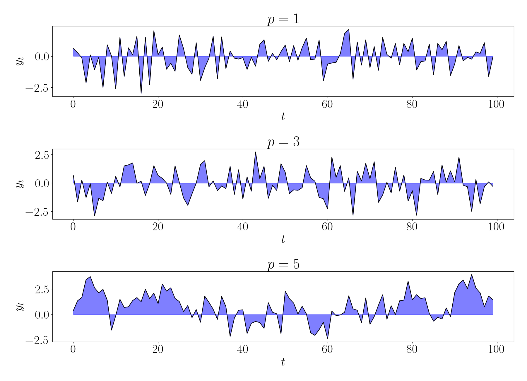
Below, we show random draws from $AR$ models with $p \in \{1, 3, 5\}.$
Covariance function
Consider two observations $y_t$ and $y_{t^\prime},$ and without loss of generality, assume that $t > t^\prime.$ The covariance between these observations under an $AR(1)$ model is then
\begin{align} \text{cov}(y_t, y_{t^\prime}) &= \mathbb{E}[y_t y_{t^\prime}] \\ &= \mathbb{E}[(\beta y_{t-1} + \epsilon_t) y_{t^\prime}] \\ &= \beta \mathbb{E}[y_{t-1} y_{t^\prime}] + \mathbb{E}[\epsilon_t y_{t^\prime}] \\ &= \beta \text{cov}(y_{t-1}, y_{t^\prime}). \end{align}
We can recursively unravel this expression $|t-t^\prime|$ times (now accounting for the case where $t^\prime > t$) to obtain
\begin{equation} \text{cov}(y_t, y_{t^\prime}) = \beta^{|t-t^\prime|} \mathbb{E}[y_{t^\prime}^2]. \tag{2} \label{eq:arcov} \end{equation}
Due to the assumption of stationarity, we know that $\mathbb{E}[y_{t^\prime}^2] = \mathbb{E}[y_{t}^2].$ We can simplify the variance of $y_{t^\prime}$ as
\begin{align} \mathbb{E}[y_t^2] &= \mathbb{E}[(\beta y_{t-1} + \epsilon_t) (\beta y_{t-1} + \epsilon_t)] \\ &= \beta^2 \mathbb{E}[y_{t-1}^2] - 2\beta \mathbb{E}[y_{t-1}] + \mathbb{E}[\epsilon_t^2] \\ &= \beta^2 \mathbb{E}[y_{t-1}^2] + \sigma^2. \end{align}
Again using the stationarity assumption, we notice that $\mathbb{E}[y_{t-1}^2] = \mathbb{E}[y_t^2].$ This yields the final expression for the variance of $y_t:$
\[\mathbb{V}[y_t] = \frac{\sigma^2}{1 - \beta^2}.\]Plugging this into Equation \ref{eq:arcov}, we obtain
\[\text{cov}(y_t, y_{t^\prime}) = \beta^{|t-t^\prime|} \frac{\sigma^2}{1 - \beta^2}.\]Due to our assumption of Gaussian errors, this allows us to recognize the $AR$ model as a special case of a Gaussian process with covariance function $k(t, t^\prime)$ given by the equation above. This covariance function can be further generalized for $p>1$ (although we won’t explore it explicitly in this post).
Moving average
The moving average model with lag $q$, which we denote as $MA(q)$, is a complement to the $AR$ model. Whereas the $AR$ model assumes dependence between the observations, the $MA$ model assumes dependence between the noise terms. The $MA(q)$ model for the $t$th observation is
\[y_t = \epsilon_t + \sum\limits_{j=1}^q \phi_j \epsilon_{t - j},~~\epsilon_t \sim \mathcal{N}(0, \sigma^2).\]We can see that the previous noise terms contribute linearly to future observations. Intuitively, the motivation behind the $MA$ model is that the noise on any given time step may not be isolated to just that time step. Instead, we might expect the noise introduced at time $t$ to propagate through future time steps as well.
We can compute the distribution of $y_t.$ Since the sum of two centered Gaussian distributions is another Gaussian with the sum of the variance, we have
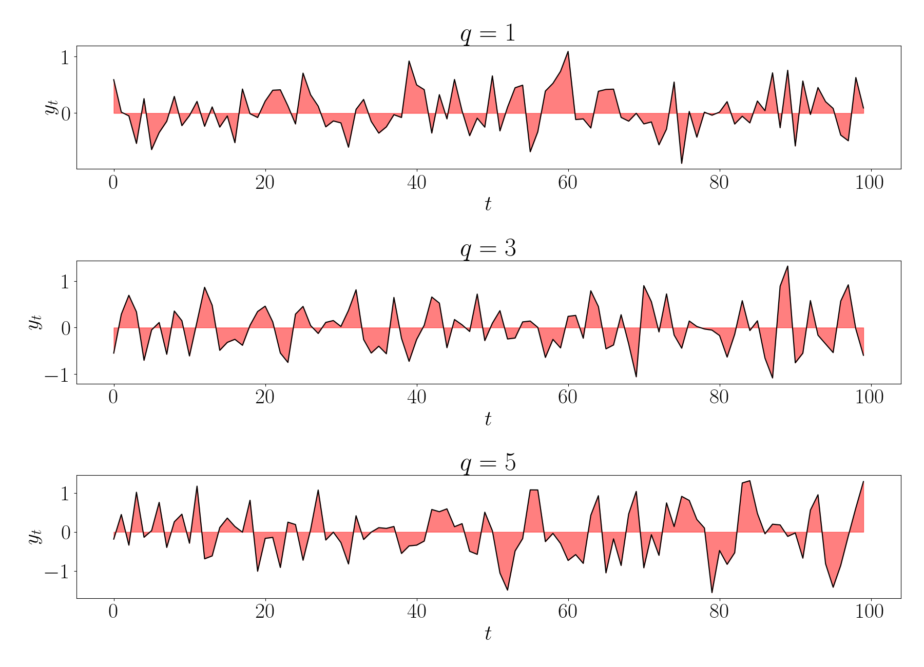
\[y_t \sim \mathcal{N}\left( 0, \sigma^2 + \sum_{j=1}^q \sigma^2 \phi_j^2 \right).\]Below, we show random draws from $MA$ models with $q \in \{1, 3, 5\}.$
Covariance function
Similar to the AR model, we can also compute the covariance between two observations $y$ and $y^\prime$ under the $MA(1)$ model. We have
\begin{align} \text{cov}(y_t, y_{t^\prime}) &= \mathbb{E}[y_t y_{t^\prime}] \\ &= \mathbb{E}[(\phi \epsilon_{t-1} + \epsilon_t) y_{t^\prime}] \\ &= \phi \mathbb{E}[\epsilon_{t-1} y_{t^\prime}] + \mathbb{E}[\epsilon_t y_{t^\prime}] \\ &= \phi^{|t - t^\prime|} \text{cov}(\epsilon_t, y_t). \end{align}
Computing this next covariance term, we have
\begin{align} \text{cov}(\epsilon_t, y_t) &= \mathbb{E}[(y_t - \phi \epsilon_{t-1}) y_t] \\ &= \mathbb{E}[y_t^2] - \phi \mathbb{E}[\epsilon_{t-1} y_t] \\ &= \mathbb{E}[y_t^2] - \phi \mathbb{E}[\epsilon_{t-1} (\phi \epsilon_{t-1} + \epsilon_t)] \\ &= \mathbb{E}[y_t^2] - \phi^2 \mathbb{E}[\epsilon_{t-1}^2] \\ &= \mathbb{E}[y_t^2] - \phi^2 \sigma^2. \end{align}
Finally, let’s simplify the variance of $y_t$ as
\begin{align} \mathbb{E}[y_t^2] &= \mathbb{E}[(\phi \epsilon_{t-1} + \epsilon_t) (\phi \epsilon_{t-1} + \epsilon_t)] \\ &= \phi^2 \sigma^2 + \sigma^2. \end{align}
Putting these pieces together, we have
\[\text{cov}(y_t, y_{t^\prime}) = \phi^{|t - t^\prime|} \sigma^2.\]Thus, we see that the $MA$ model is also a special case of a Gaussian process with a covariance function given by the equation above.
ARMA
Putting the $AR$ and $MA$ models together, the $ARMA(p, q)$ model assumes both a dependence directly between the observations, as well as the noise. The $ARMA(p, q)$ model is given by
\[y_t = \epsilon_t + \sum\limits_{i=1}^p \phi_i y_{t - i} + \sum\limits_{j=1}^q \beta_j \epsilon_{t - j}.\]The benefit of ARMA models is that they can capture stable trends in a time series through the AR model, as well as short-term “shocks” in the trend through the MA model.
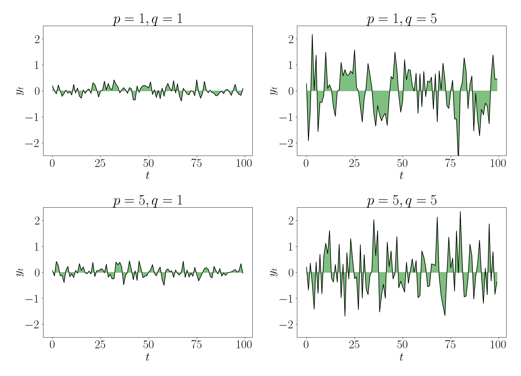
Below, we show random draws from $MA$ models with $p, q \in \{1, 5\}.$