ARMA distributions

\(\DeclareMathOperator*{\argmin}{arg\,min}\) \(\DeclareMathOperator*{\argmax}{arg\,max}\)

Autoregressive and moving average models are commonly used for time series data. While these models are usually presented as a recursive regression, they’re less frequently shown in terms of their assumptions of the marginal distribution of each sample. Here, we derive the distributional assumptions underlying these models. We show this for the AR(1) model, the MA(q) model, and the ARMA(1, q) model.

AR(1) model

Consider a set of time-ordered samples $x_1, x_2, \dots, x_T$ whose behavior over time we wish to model. Recall the AR(1) model:

where $\beta$ is the autoregressive parameter, and $\epsilon_t$ is a noise term. Let’s compute the distribution for $x_t$ incrementally. Given an initial point $x_1$, let’s unravel the recursive model definition for $t=2, \dots$ as follows:

\begin{align} x_t &= \beta x_{t-1} + \epsilon_t \\ &= \beta \color{red}{(\beta x_{t-2} + \epsilon_{t-1})} + \epsilon_t \\ &= \beta \color{red}{(\beta \color{blue}{(\beta x_{t-3} + \epsilon_{t-2})} + \epsilon_{t-1})} + \epsilon_t \\ &= \beta \color{red}{(\beta \color{blue}{(\beta \color{green}{(\beta x_{t-4} + \epsilon_{t-3})} + \epsilon_{t-2})} + \epsilon_{t-1})} + \epsilon_t \\ &= \beta^{t-1} x_{1} + \epsilon_t + \beta \epsilon_{t-1} + \beta^2 \epsilon_{t-2} + \cdots + \beta^{t-2} \epsilon_2 \\ &\quad\quad\quad\quad\vdots \\ &= \beta^{t-1} x_{1} + \sum\limits_{i=0}^{t-2} \beta^{i} \epsilon_{t-i} \\ \end{align}

Given the initial point $x_1,$ the first term, $\beta^{t-1} x_{1},$ will be a constant. Each term in the second term’s sum is a Gaussian random variable multiplied by a constant. We know that $\beta^{i} \epsilon_{t-i} \sim N(0, \beta^{2i} \sigma^2).$ Since the $\epsilon$ terms are i.i.d., the variances are additive; thus, the distribution for $x_t$ for $t \geq 2$ is given by

We can examine the behavior of $x_t$ as we extend to an infinite time horizon, $t \to \infty.$ Examining the mean, we have three cases depending on the value of $\beta:$

• If $|\beta| < 1$, then $\beta^{t-1} x_1 \to 0$ as $t \to \infty;$
• If $|\beta| > 1$, then $\beta^{t-1} x_1 \to \infty$ as $t \to \infty;$
• If $|\beta| = 1$, then $\beta^{t-1} x_1 = x_1$ for all $t.$

In other words, the mean converges to zero, diverges to infinity, or remains constant at the initial value depending on whether the autoregressive parameter’s absolute value is less than, greater than, or equal to one, respectively.

For the variance, we can notice that it takes the form of a geometric series and thus the infinite sum has a closed form when $|\beta| < 1:$

When $\beta = 1,$ the AR(1) model reduces to the vanilla Wiener process (often called a random walk), where the variance of $x_t$ scales directly proportionally to $t.$

We show a small demonstration of this distribution below. We simulate data for $T=100$ steps with $\beta = 0.9$ and $\sigma^2 = 0.01.$ We repeat this 10,000 times and plot a histogram of the values of $x_{100}$ in gray. We also plot the limiting distribution of $x_t$ as a red dashed line.

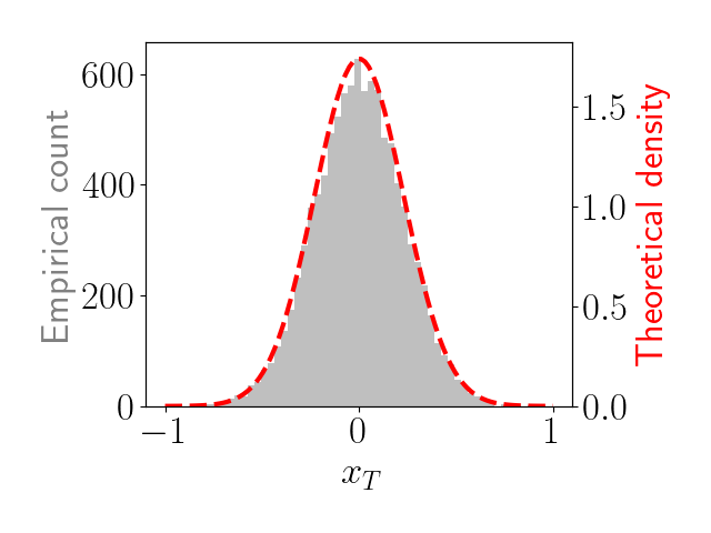
We can see that the gray density (the one we observe empirically by sampling from the model) closely matches the theoretical limiting density (the one that will be approached with an infinite time horizon).

The Python code for this experiment is below.

import numpy as np
import matplotlib.pyplot as plt
from scipy.stats import norm

beta = 0.9
sigma2 = 1e-2
n = 100
X = np.zeros(n)
n_repeats = 2000
last_xs = np.zeros(n_repeats)

for nn in range(n_repeats):

    for ii in range(1, n):
        X[ii] = X[ii - 1] * beta + np.random.normal(
            scale=np.sqrt(sigma2)
        )

    last_xs[nn] = X[-1]

theoretical_mean = 1 / (beta ** (n - 1)) * X[0]
theoretical_variance = sigma2 * (1 / (1 - beta**2) - 1)
lim = 1
xs = np.linspace(-lim, lim, 100)
ps = norm.pdf(
    xs, 
    loc=theoretical_mean, 
    scale=np.sqrt(theoretical_variance))

plt.hist(last_xs, 50, color="gray", alpha=0.5)
plt.xlabel(r"$x_T$")
plt.ylabel("Empirical count", color="gray")

ax = plt.gca().twinx()
ax.plot(xs, ps, c="red", linestyle="--", linewidth=3)
ax.set_ylim([0, ax.get_ylim()[1]])
ax.set_ylabel("Theoretical density", color="red")
plt.show()

MA(q) model

Let’s next consider the MA(1) model for our data $x_1, \dots, x_T:$

Since $x_t$ is a sum of two i.i.d. Gaussian random variables, the distribution of $x_t$ is easily derived. Given the variances of each of the two terms, $\mathbb{V}[\alpha \epsilon_{t-1}] = \alpha^2 \sigma^2$ and $\mathbb{V}[\epsilon_{t}] = \sigma^2,$ we have the following distribution for $x_t$ for all $t$:

Thus, the distribution of $x_t$ is constant across all time steps and does not depend on $t.$

This analysis can be easily generalized to the $\text{MA}(q)$ model, where the $t$th sample depends on the previous $q$ error terms:

Again, $x_t$ is simply a weighted sum of i.i.d. Gaussian random variables, where $\mathbb{V}[\alpha_j \epsilon_{t-1}] = \alpha_j^2 \sigma^2.$ This implies that the distribution of $x_t$ is given by

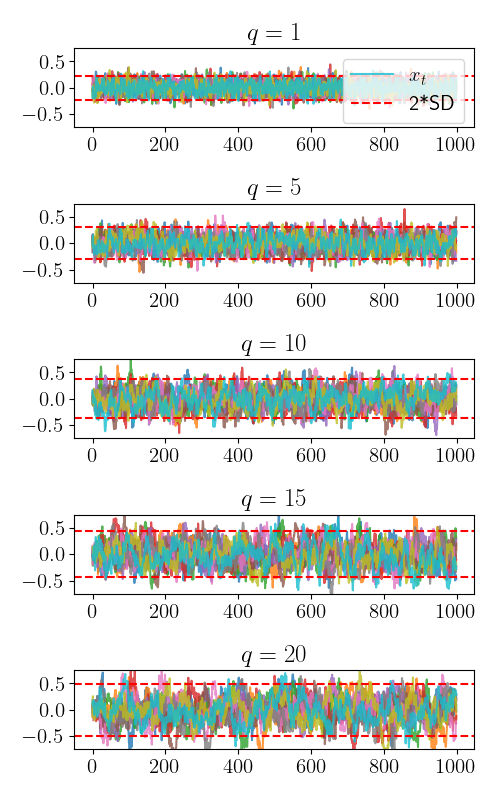
Intuitively, this means that the variance of $x_t$ will be higher for larger $q$ (and of course, will be higher for larger $\alpha_j$ as well).

We demonstrate this empirically below. We plot multiple draws from the MA(q) model with $q \in {1, 5, 10, 15, 20}.$ The horizontal dashed lines show twice the theoretical standard deviation.

ARMA model

Finally, let’s consider the ARMA(1, 1) model:

In the previous two sections, we have derived the distributions for each of these terms:

This leaves us with the following resulting distribution for $x_t$ under the ARMA(1, 1) model:

Similarly, for the ARMA(1, q) model, the distribution has a simple extension:

References

• Shumway, Robert H., and David S. Stoffer. Time series analysis and its applications. Vol. 3. New York: springer, 2000.