Andy Jones
False discovery rate and the $q$-value
\(\DeclareMathOperator*{\argmin}{arg\,min}\) \(\DeclareMathOperator*{\argmax}{arg\,max}\)
Multiple hypothesis testing requires balancing multiple types of errors and determining a tolerable level of such errors. One of the most common approaches to this problem controls the probability of seeing at least one false positive (known as the the family-wise error rate); however, this can be overly restrictive if one is testing many hypotheses and wants to ensure that interesting findings are not missed. To circumvent this problem, scientists often control the fraction of discoveries that are incorrect (known as the false discovery rate) instead. Use of this error control approach typically allows for more findings to be discovered, while restricting the number of false positives.
In this post, we first review the basics of statistical hypothesis testing, and then we describe the false discovery rate (FDR). We finish by describing an alternative to the $p$-value that is concerned with the FDR, called the $q$-value.
Hypothesis testing
We consider the setting in which we test a simple hypothesis:
\[H_0: \theta = \theta_0,~~~H_1: \theta \neq \theta_0\]where $\theta \in \Theta$. Our goal in hypothesis testing is to construct a decision rule for when to reject the null hypothesis. Given some data $X = (x_1, \dots, x_n)$, we must construct two quantities to carry out the test:
- A test statistic $T(X)$, which will provide our summary of the data,
- A critical region $\mathbb{C} \subseteq \Theta$ (also known as a rejection region), which will determine when we reject $H_0$.
Given these quantities, our decision rule is to reject $H_0$ if the test statistic falls in the critical region:
\[\text{Reject $H_0 \iff T(X) \in \mathbb{C}$}.\]There are two types of errors that we can make, as demonstrated by this contingency table:
| Accept $H_0$ | Reject $H_0$ | |
|---|---|---|
| $H_0$ true | ✅ | Type I error |
| $H_1$ true | Type II error | ✅ |
A $p$-value is a measure of how frequently we expect to incorrectly reject the null hypothesis when the null hypothesis is true ($\theta = \theta_0$). Letting $p_{\theta_0}$ denote the distribution under the null hypothesis, we can write a p-value as:
\[p_{\theta_0}(\text{Reject $H_0$}) = p_{\theta_0}(T(x) \in \mathbb{C}).\]Simple example
Consider a dataset $x_1, \dots, x_n$, which we model as $x_i \sim \mathcal{N}(\mu, \sigma^2)$ where $\sigma^2$ is known. Suppose we wish to test the following hypothesis:
\[H_0: \mu \leq 0,~~~H_1: \mu > 0.\]A reasonable test statistic is the sample average $T(X) = \bar{X} = \frac1n \sum_{i=1}^n x_i$. In this case, we know the exact distribution of $T(X)$:
\[\bar{X} \sim \mathcal{N}(\mu, \sigma^2 / n).\]Of course, we don’t know $\mu$ in practice, but we know that under the null hypothesis,
\[\bar{X} \sim \mathcal{N}(0, \sigma^2 / n).\]To control the Type I error of our test at level $\alpha$, we want to find a critical value $c$ such that
\[p_{\theta_0}(\bar{X} > c) \leq \alpha.\]In most real-world settings, scientists choose $\alpha = 0.05$ or $\alpha = 0.01$.
We can transform $\bar{X}$ so that its distribution is standardized. In particular, if the null hypothesis were true, it holds that $\mu = 0$, and $\frac{\sqrt{n}}{\sigma} \bar{X}$ then follows a standard normal. Transforming both sides of the inequality, we have:
\[p_{\theta_0}\left(\underbrace{\frac{\sqrt{n}}{\sigma} \bar{X}}_{\sim \mathcal{N}(0, 1)} > \frac{\sqrt{n}}{\sigma} c\right) \leq \alpha.\]We can notice that the left hand side is equal to $1 - \Phi(c \sqrt{n} / \sigma)$, where $\Phi(\cdot)$ is the CDF for the standard normal. Thus, we can see that our critical value must be
\[c = 1 - \Phi^{-1}(\alpha).\]Below, we illustrate this test. Suppose that the real data generating distribution is $\mathcal{N}(1, 1)$. Note that this distribution is unknown, but we observe samples from it. Here, we draw $n = 5$ samples from the data distribution and test the hypothesis $H_0: \mu \leq 0, H_1: \mu > 0$.
The solid line shows the distribution of the test statistic $\bar{X}$ under the null hypothesis, and the dashed line shows the distribution of $\bar{X}$ under the true (unobserved) data distribution. The vertical dotted line indicates the critical value. We show the regions determining type I error in green and the type II error in red.
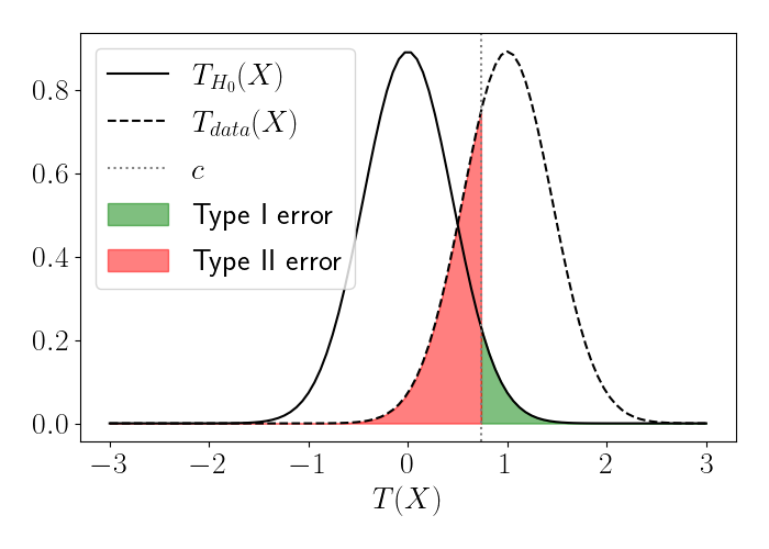
Clearly, if we were to make our critical value $c$ even larger, we would decrease the Type I error, but this would come at the cost of greater Type II error. These tradeoffs become critical when thinking about testing many hypotheses simultaneously, which we explore next.
Multiple hypothesis testing
In many scientific settings, we test several hypothesis tests at once. If we carry over our procedure above and test $M$ hypotheses, each at level $\alpha$, then our overall type I error rate will be
\[p_{\theta_0}\left(\bigcup\limits_{m=1}^M \text{Reject $H_0^m$}\right) = 1 - p_{\theta_0}\left(\bigcap\limits_{m=1}^M \text{Accept $H_0^m$}\right) = 1 - (1 - \alpha)^M,\]where $H_0^m$ is the null hypothesis corresponding to hypothesis $m$. As $M$ becomes large, our Type I error will increase as well. For example, testing $M = 20$ hypotheses at level $\alpha = 0.05$ already implies an overall Type I error rate of 0.64, even though each individual test has a Type I error of 0.05. Thus, there’s a need to control error more conservatively when we run multiple tests.
Similar to our table above, we can enumerate all possible outcomes for our multiple hypothesis testing problem. Below, each cell shows the number of hypotheses that fall into each category.
| Accept $\mathbf{H_0}$ | Reject $\mathbf{H_0}$ | ||
|---|---|---|---|
| $\mathbf{H_0}$ true | A | B | C = A + B |
| $\mathbf{H_1}$ true | D | E | F = D + E |
| G = A + D | H = B + E | M = G + H = C + E |
Note that only $G$, $H$, and $M$ are observed, and the rest of the quantities are unknown.
Family-wise error rate
One of the most common ways to deal with the multiple hypothesis testing problems is to control the family-wise error rate (FWER). The FWER is defined as the probability of incorrectly rejecting at least one of the null hypotheses:
\[FWER = p_{\theta_0}(B \geq 1).\]The most straightforward procedure to control the FWER is known as the Bonferroni correction. If we wish to control the FWER at error level $\alpha$, then we can test each individual hypothesis at level $\alpha / M$. To see this, we can bound the probability that we obtain at least one incorrect rejection. Let $H_0^m$ be the null hypothesis for the test $m$. Then we have
\begin{align} p_{\theta_0}\left(\bigcup_{m=1}^M \text{Reject $H_0^m$}\right) &\leq \sum\limits_{m=1}^M p_{\theta_0}(\text{Reject $H_0^m$}) & \text{(Union bound)} \\ &= \sum\limits_{m=1}^M \alpha / M \\ &= \alpha. \end{align}
While this correction is appealing for its simplicity, it can be extremely restrictive, especially as the number of hypotheses becomes large. Controlling the possibility of at least one incorrect rejection is very strict, and it requires a very low error tolerance when $M$ is large. For example, if we were to run $20,000$ tests (the number of genes in the human genome) while controlling the FWER at level $\alpha$, then we would only reject the null hypothesis with a $p$-value of at least $0.05 / 20,000 = 0.0000025$. If we have potential findings that don’t meet this strict threshold, we may miss important results.
We next explore one strategy to circumvent this issue.
False discovery rate
As mentioned above, controlling the FWER may limit the number of findings we discover and can overly inflate our Type II error. If we’re testing lots of hypotheses, we may be willing to tolerate some fraction of false rejections, rather than tolerating only the possibility that there are any false rejections.
This is the basic idea behind the False Discovery Rate (FDR): controlling the fraction of rejections that are incorrect. More precisely, using the notation defined in the table above, we can define the FDR as follows:
\[FDR = \mathbb{E}\left[\frac{B}{H}\right] = \mathbb{E}\left[ \frac{\text{# false rejections}}{\text{# rejections}} \right].\]Using certain procedures, we can control this quantity and ensure that we are observing interesting findings while being measured in the number of incorrect rejections we have.
FDR procedure
We next discuss the procedure proposed by Benjamini and Hochberg to control the FDR. Let $P_1, P_2, \dots, P_M$ be the p-values corresponding to $M$ hypothesis tests, and suppose they’re ordered without loss of generality, $P_1 \leq P_2 \leq \dots \leq P_M$. Then, to control the FDR at rate $\alpha$, Benjamini and Hochberg propose the following procedure:
- Set $k$ be the largest integer $m$, $1 \leq m \leq M$, for which $P_m \leq \frac{m}{M} \alpha$.
- Reject all $H_m$ for $m=1,\dots,k$.
To see why this works, let’s define a model for the $p$-values. Suppose our $p$-values come from the following mixture model:
\[G(P) = \pi_1 F_1(P) + \pi_0 F_0(P),\]where $\pi_1 = p(H = 1)$ and $\pi_0 = 1 - \pi_1 = p(H = 0)$ are the prior probabilities for the hypotheses, and $F_1$ and $F_0$ are the CDFs of the alternative hypotheses, respectively. As usual, we assume that the null p-values are uniform, so $F_0(P) = P$.
Now, we can give a sketch for how the procedure arrives at controlling the FDR. To start, suppose we decide to reject all hypotheses with $P_m \leq t$, where $t \in [0, 1]$ is a threshold. If we were to carry out this decision rule, we can approximate the corresponding FDR as follows.
\[FDR(t) = \mathbb{E}\left[ \frac{\sum\limits_{m=1}^M 1\{ P_m \leq t \} (1 - H_m) }{\sum\limits_{m=1}^M 1\{P_m \leq t\}} \right].\]For simplicity, let’s approximate the numerator and denominator separately,
\[FDR(t) \approx \frac{\mathbb{E} \left[ \sum\limits_{m=1}^M 1\{ P_m \leq t \} (1 - H_m) \right]}{\mathbb{E} \left[\sum\limits_{m=1}^M 1\{P_m \leq t\} \right]}.\]Finally, we can switch the sum and expectation and evaluate known quantities:
\begin{align} FDR(t) &\approx \frac{ \sum\limits_{m=1}^M \mathbb{E}\left[ 1\{ P_m \leq t \} | H_m = 0 \right] p(H_m = 0)}{\sum\limits_{m=1}^M \mathbb{E} \left[ 1\{P_m \leq t\} \right]} \\ &= \frac{M \pi_0 t}{M G(t)} \\ &= \frac{\pi_0 t}{G(t)} \end{align}
If we let $\pi_0 = 1$ and estimate $G(t)$ with the empirical CDF, $\widehat{G}(t) = \frac1M \sum_{m=1}^M 1\{P_m \leq t\}$, then for each of our observed p-values, we have
\[\widehat{G}(P_k) = \frac1M \sum\limits_{m=1}^M 1\{P_m \leq P_k\} = \frac{k}{M}.\]Considering our procedure again, we have
\begin{align} \max \left\{k : P_k \leq \frac{k}{M} \alpha\right\} &= \max \left\{k : P_k \leq \widehat{G}(P_k) \alpha\right\} \\ &= \max \left\{k : \frac{P_k}{\widehat{G}(P_k)} \leq \alpha\right\}. \\ \end{align}
Thus, one way to see this procedure is as approximating the distribution of $p$-values $G$ with its empirical CDF and setting $\pi_0 = 1$. See Benjamini and Hochberg for a more rigorous and complete proof of why the procedure works.
$q$-value
One of the downsides of the FDR is the awkwardness in interpretation. Like a $p$-value, using an FDR requires first fixing an error rate and then estimating the corresponding rejection region. However, if we fix an overly restrictive error rate, we may not find as many discoveries as we had hoped. Thus, it can make more sense to first fix a rejection region and then estimate the corresponding error rate if we were to reject all hypothesis test statistics that fall in that region.
When we use FDRs, we typically want to find many rejections (and typically have a higher tolerance for error), so fixing an error rate a priori may lead to only a small number of hypotheses being rejected.
This is the motivation for the $q$-value, as developed by John Storey in a 2002 paper.
To be more precise about our explanation above, notice that we can rewrite our expression for a $p$-value as
\[p\text{-value}(t) = p(T \geq t | H = 0).\]In a $p$-value approach, we fix a tolerable error rate $\alpha$ and reject all hypotheses with a $p$-value less than $\alpha$. Similarly, with an FDR approach, we may fix a tolerance level for the FDR, and then reject all hypotheses such that this tolerance is met.
The $q$-value reverses this process. Suppose we decide how many (or what fraction of) hypotheses we want to reject, and then estimate how many false discoveries we should expect to incur. In other words, the $q$-value reverses the conditional probability above:
\[q\text{-value}(t) = p(H = 0 | T \geq t).\]In plain words, the $q$-value asks: Given that we rejected a null hypothesis, what is the probability that this null hypothesis was actually true? For example, this approach would allow us to reject the hypotheses with the $100$ lowest $p$-values, and then estimate what fraction of these we should expect to be false positives.
To see the $q$-value in a slightly different light, we can expand the $q$-value expression, and see
\begin{align} p(H = 0 | T \geq t) &= \frac{p(T \geq t | H = 0) p(H = 0)}{p(T \geq t)} \\ &= \frac{p(T \geq t | H = 0) \pi_0}{p(T \geq t | H = 0) \pi_0 + p(T \geq t | H = 1) \pi_1}. \end{align}
Thus, in a Bayesian sense, the $q$-value can be seen as a sort of posterior probability of a $p$-value, where we place a prior $\pi_0$ on the probability of a null hypothesis being true.
In this post, we won’t explore the details of how to compute a $q$-value in practice, but we can gain intuition for what the $q$-value is measuring using the following animation.
The above movie shows the histogram of $p$-values that results from running the Gaussian mean test with $\pi_0 = \pi_1 = 0.5$. Notice that when the alternative mean is close to $0$, the distribution of $p$-values is uniform. Then, as the mean of the alternative distribution moves farther away from $0$, the $p$-values become more sharply peaked around $0$.
Procedures to compute a $q$-value essentially uses this empirical distribution of $p$-values to estimate the quantities of interest. We can use the fact that the $p$-values corresponding to the null hypothesis are uniformly distributed to estimate $\pi_0$. Then, we can get an estimate of the $q$-value.
References
- Benjamini, Yoav, and Yosef Hochberg. “Controlling the false discovery rate: a practical and powerful approach to multiple testing.” Journal of the Royal statistical society: series B (Methodological) 57.1 (1995): 289-300.
- Storey, John D. “A direct approach to false discovery rates.” Journal of the Royal Statistical Society: Series B (Statistical Methodology) 64.3 (2002): 479-498.
- Storey, John D. “The positive false discovery rate: a Bayesian interpretation and the q-value.” The Annals of Statistics 31.6 (2003): 2013-2035.
- Christopher Genovese’s slides on FDR.