Empirical Bayes

\(\DeclareMathOperator*{\argmin}{arg\,min}\) \(\DeclareMathOperator*{\argmax}{arg\,max}\)

Bayesian inference requires the analyst to carefully state their modeling assumptions. One of the central steps in specifying a model is choosing prior distributions for parameters of interest. However, this step is one of the most controversial parts of Bayesian methodology: Selecting priors can be a highly subjective exercise, and it’s often difficult to justify choosing one prior over another.

Empirical Bayesian approaches try to partially alleviate this issue by selecting priors using the data itself. At first, this can sound antithetical to the Bayesian mindset: Priors should be set before observing any data (it’s in the name after all). However, empirical Bayesian analysis can help modelers choose more useful priors, and it turns out to have some nice properties.

In this post, we give two simple example applications of empirical Bayes methods.

Gaussian example

Suppose we have a dataset with $p$ features, and we have $n$ observations for each feature. Let $x_{ij}$ be the $i$th observation of the $j$th feature. Now, let’s suppose we’re interested in estimating the mean of each feature, $\mu_j = \mathbb{E}[x_{ij}]$ for $j = 1,\dots,p$.

As a more concrete example, in a gene expression study we may have collected measurements on the expression level of $p$ genes, with $n$ replicates of each. In this case, the replicates may be from different biological or technical replicated samples, which we assume to be drawn from the same underlying population. Then we might be interested in estimating the mean expression value of each gene in this population. In real world studies, typical values for the number of replicates can be around $3$ to $5$. With a low number of observations for each gene, it’s difficult to robustly estimate a full posterior for the mean of each gene. However, with an empirical Bayes approach, we can share information across genes to get a better estimate.

Consider the following two-stage hierarchical model for this dataset:

\begin{align} x_{ij} &\sim \mathcal{N}(\mu_j, \sigma^2) \\ \mu_j &\sim \mathcal{N}(\mu_0, \sigma^2_0), \end{align}

where $\mu_0$ and $\sigma^2_0$ are the parameters of the prior distribution. For simplicity, let’s assume that the likelihood variance is known to be $\sigma^2=1$. To reiterate, we’re interested in computing the posterior $p(\mu_j | x_{1j}, \dots, x_{nj})$.

In a typical Bayesian setting, the analyst would choose $\mu_0$ and $\sigma^2_0$ in order to fully specify the prior. This is typically done using prior knowledge about the domain, although it’s far from a perfect science. Choosing these prior parameters is a controversial step in Bayesian data analysis, as the choices are often not given full justification.

Once the prior is set, we can compute the posterior for $\mu_j$ using the closed-form Gaussian posterior:

Taking an empirical Bayesian approach, we could instead choose $\mu_0$ and $\sigma^2_0$ based on the data itself. In particular, if we assume that the features $j=1,\dots,p$ are somehow related to one another, we can share information across the features so that we have a more robust estimate of the mean for each individual feature. Returning to the gene expression example, this means that we assume that all genes are expected to be drawn from some underlying distribution over gene expression. It’s not clear a priori what the mean and variance of this gene distribution looks like, so we can use our observed data to learn about it.

A straightforward empirical Bayesian approach is to set the prior paramters with the observed mean and variance in the data itself. In particular, let $\bar{x}_j = \frac{1}{n_j} \sum_{i=1}^{n} x_{ij}$.

To see how this would work, let’s first generate some data with the code below. We use $p=20,000$ features (approximately the number of genes in the human genome).

import numpy as np

## Data generation settings
n_replicates = 3
true_prior_mean = 10
true_prior_variance = 1.
data_var = 1.
n_features = 20000

## Generate means from bottom of hierarchy
means = np.random.normal(loc=true_prior_mean, 
             scale=np.sqrt(true_prior_variance),
             size=n_features)

## Generate data from second rung of hierarchy
X = np.random.normal(loc=np.repeat(means.reshape(1, -1), 
           n_replicates, axis=0), 
           scale=data_var, 
           size=(n_replicates, n_features))

## Compute observed mean of each feature (MLE)
observed_means = X.mean(0)

A histogram of our data’s empirical means is below.

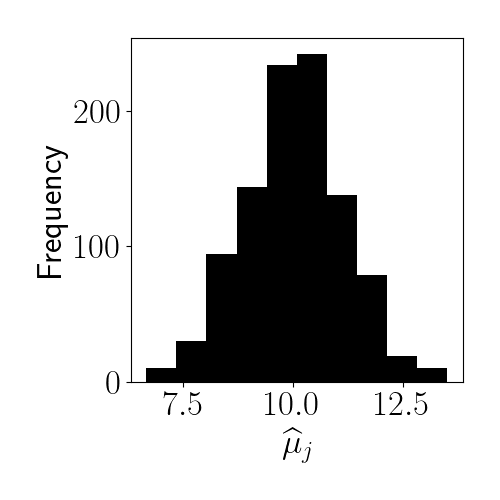
Then we can set the prior parameters as follows:

The following code computes these parameters for our data:

## Prior parameter for empirical Bayes model
eb_prior_mean = np.mean(observed_means)
eb_prior_var = np.var(observed_means)

## In the Bayesian approach, we choose these parameters manually
bayes_prior_mean = 0
bayes_prior_var = 1

## Functions for Bayesian posterior for each feature
def gaussian_posterior_mean(x, prior_mean):
  return (x.sum() + prior_mean) / (len(x) + 1)

def gaussian_posterior_var(x, prior_var, data_var):
  return 1 / (1 / prior_var + 1 / (data_var / len(x)))

## Standard Bayes
bayes_posterior_means = [gaussian_posterior_mean(X[:, jj], bayes_prior_mean) for jj in range(n_features)]
bayes_posterior_variances = [gaussian_posterior_var(X[:, jj], bayes_prior_var, data_var) for jj in range(n_features)]

## Empirical Bayes
ebayes_posterior_means = [gaussian_posterior_mean(X[:, jj], eb_prior_mean) for jj in range(n_features)]
ebayes_posterior_variances = [gaussian_posterior_var(X[:, jj], eb_prior_var, data_var) for jj in range(n_features)]

Here, we obtain the following estimates:

For comparison, let’s also fit a standard Bayesian model where we assume that the prior parameters are given by $\mu_0 = 0, \sigma^2_0 = 1$. A default prior mean of zero is not uncommon, but in this case it drastically underestimates the true prior mean of the data.

Let’s visualize the difference between standard Bayes and empirical Bayes in this setup. In the left two panels below, we plot the true underlying means against 1) the standard Bayes posterior means and 2) the empirical Bayes posterior means. In the right panel, we plot the empirical Bayes posterior means against the maximum likelihood estimate (MLE) of each feature. In this case, the MLE is just the sample average, $\widehat{\mu}_j$.

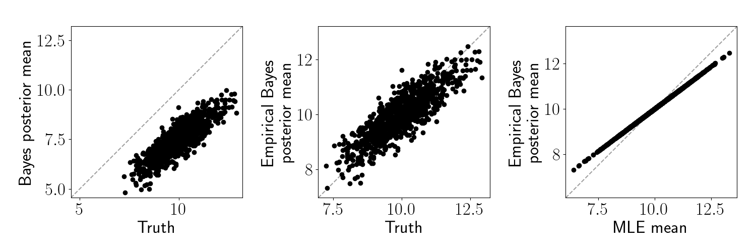
We can see that the posterior mean for the standard Bayesian approach is biased downward because our prior mean was set too low. In contrast, the empirical Bayes sets an appropriate prior and thus much more closely matches the truth. Moreover, we can see that the empirical Bayes estimate regularizes the MLE toward the prior mean.

Differing numbers of replicates

To make the situation slightly more interesting, suppose we have a different number of replicates for each feature. Specifically, let feature $j$ have $n_j$ replicates.

In this case, we expect samples with more replicates to rely on the prior less since more data is available. Here, the information-sharing between features becomes especially powerful because features with very few replicates can leverage information from features with lots of replicates.

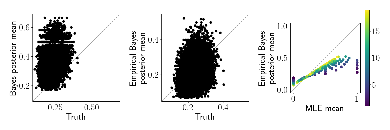
Here, we generate the same dataset as above, but randomly select the number of replicates for each feature from ${1, 2, \dots, 20}$. We perform the same analysis as above. Below, we make the same plots as above, but color each point by the number of replicates for that feature.

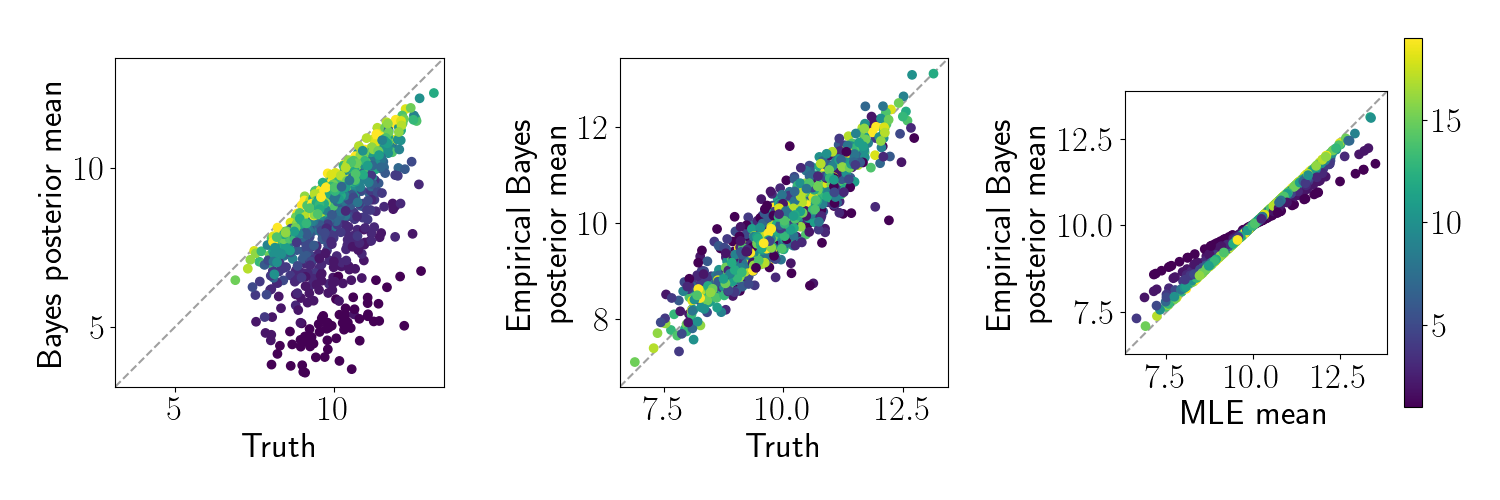
As expected the features with fewer samples are regularized more heavily toward the prior mean. However, while the standard Bayes approach regularizes the estimates toward zero, the empirical Bayesian approach regularizes them toward the empirical mean.

Beta-Bernoulli example

Let’s next consider a non-Gaussian (yet still simple) example. This example is inspired by David Robinson’s post on empirical Bayes.

Suppose we have $n$ two-sided coins, each of which shows either heads or tails on a given flip. Let $x_{ij} = 1$ represent heads and $x_{ij} = 0$ represent tails for the $j$th flip of coin $i$. Consider a beta-Bernoulli model for these data:

\begin{align} x_{ij} &\sim \text{Bern}(\theta_j) \\ \theta_j &\sim \text{Beta}(\alpha_0, \beta_0), \end{align}

where $\alpha_0$ and $\beta_0$ are our prior parameters. We’re interested in the posterior for the frequency of heads for each coin, $p(\theta_j | x_{1j}, \dots, x_{n_j j})$.

In the standard Bayesian setting, we would choose values for the prior parameters manually, and then form the posterior for each $\theta_j$. The posterior again has a closed form in this conjugate model:

Alternatively, taking an empirical Bayesian approach, we can estimate $\alpha_0$ and $\beta_0$ from the observed distribution of coin flips.

Let’s start by generating data with the following code:

import numpy as np

true_prior_a = 70
true_prior_b = 200
n_features = 20000
n_replicates = np.random.choice(np.arange(1, 20), size=n_features, replace=True)

thetas = np.random.beta(a=true_prior_a, b=true_prior_b, size=n_features)
X = [np.random.binomial(n=1, p=thetas[jj], size=n_replicates[jj]) for jj in range(n_features)]

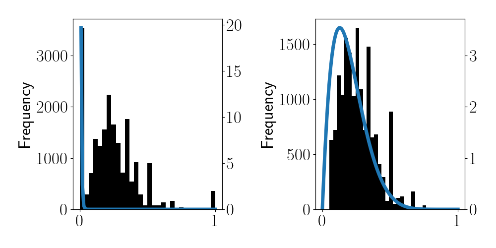
Let $\bar{x}_j = \frac{1}{n_j} \sum_{i=1}^{n_j} x_{ij}$ be the observed frequency of heads for each coin. Below is a histogram for these values for our dataset:

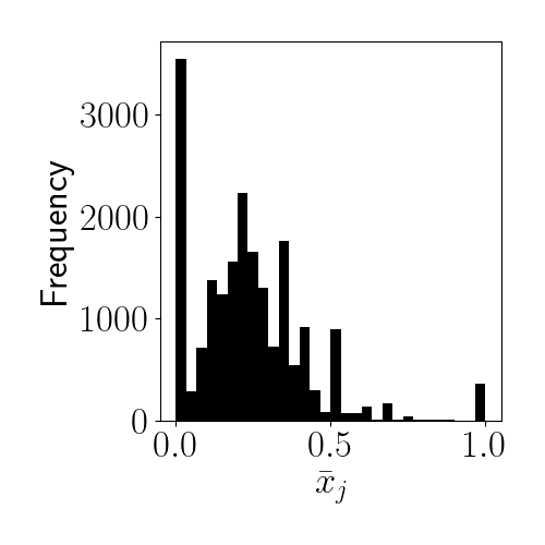
We can see that most of the coins are slightly biased toward $0$ (tails). Also, notice that there are many coins whose observed frequencies of heads or tails is either exactly $0$ or $1$. The maximum likelihood estimate for these coins would thus be $\widehat{\theta}_j = 0$ or $\widehat{\theta}_j = 1$, indicating that the coin is entirely biased toward tails or heads. However, these edge cases arise because coins with extreme MLEs tend to have been flipped very few times. For example, if a certain coin was flipped just once, the MLE would necessarily be either $0$ or $1$. Instead, we’d like to regularize these estimates.

Instead of the standard Bayesian approach (in which we’d select the priors beforehand), here we’ll take an empirical Bayesian approach and share information across coins. This is useful here because we can leverage information from coins that have been flipped many times to better inform our estimates for coins that have only been flipped once or twice.

To enable empirical Bayesian inference, let’s directly fit a beta distribution via maximum likelihood on this set of observed frequencies in the histogram above.

import numpy as np
from scipy.stats import beta

observed_means = [x.mean() for x in X]
a_mle, b_mle, _, _ = beta.fit(observed_means)

We find the following values:

The PDF of a beta is plotted in blue in the left panel below. It seems clear that the MLE is being thwarted by the extreme values of frequencies. For this reason, let’s try to exclude coins that show an empirical frequency of either $0$ or $1$. The right panel below shows this alternate beta PDF, which has $\widehat{a}_0 = 3.95,\widehat{b}_0 = 6.13$.

Now, let’s use these empirical estimates for the prior parameters to do our downstream inference on each $\theta_j$. We compare to a Bayesian procedure that assumes that $\alpha_0 = 5, \beta_0 = 5$.

Below, we can see that neither the standard Bayes nor the empirical Bayes posterior recovers the true $\theta_j$ very well. However, note that the empirical Bayes procedure regularizes the extreme values back to the observed mean.

Conclusion

Empirical Bayesian analysis can guide the choice of prior distribution when there is little prior knowledge, and it can also enable information sharing across seemingly unrelated samples, making the final posterior more accurate and robust.

References

• Smyth, Gordon K. “Linear models and empirical bayes methods for assessing differential expression in microarray experiments.” Statistical applications in genetics and molecular biology 3.1 (2004).
• Casella, George. “An introduction to empirical Bayes data analysis.” The American Statistician 39.2 (1985): 83-87.
• David Robinson’s book, Introduction to Empirical Bayes: Examples from Baseball Statistics.
• David Robinson’s post on empirical Bayes.