Andy Jones
Effective sample size
\(\DeclareMathOperator*{\argmin}{arg\,min}\) \(\DeclareMathOperator*{\argmax}{arg\,max}\)
Statistical theories and models often assume that a collection of random variables are independent and identically distributed (i.i.d.). However, this assumption is often false in practice.
In Bayesian statistics, one setting where this appears is in MCMC approaches for posterior infrerence. In many of these situations, we have long sequences of random variables that exhibit correlation structure across time (samples drawn more closely to one another tend to be correlated). In order to properly characterize the error in the estimates we derive from these approaches, we cannot simply treat these samples as independent, as this would underestimate our error. Instead, we have to account for this correlation.
The effective sample size is a metric that measures how much information content is loss due to the correlation in the sequence. In other words, although our sequence may have a length (sample size) of $N$, our effective sample size will be smaller due to the correlation and redundancy between the samples. Below, we review the CLT, and then explain autocorrelation and the effective sample size metric.
Central limit theorem
Let’s recall the central limit theorem (in informal terms). Suppose we have a sequence of $N$ random variables $X_1, X_2, \dots, X_N$, each of which is drawn independently from a distribution with mean $\mu$ and variance $\sigma^2$. The classical CLT tells us that the empirical average of this sequence will be Gaussian distributed:
\begin{equation} \frac1N \sum\limits_{i=1}^N X_i \to_d \mathcal{N}(\mu, \sigma^2 / N).\tag{1}\label{eq:1} \end{equation}
Correlated samples
In the classical CLT, we crucially assume that the $N$ samples are independent of one another. However, in most MCMC sampling approaches, samples drawn sequentially will be positively correlated (or autocorrelated, in the parlance of time-series) with one another. When samples exhibit autocorrelation, the sequence contains less information content about the underlying distribution in some sense. This is because the information content in any two correlated samples is partially reduntant with one another, whereas two independent samples are more likely more to provide new information about the distribution.
Furthermore, when samples are correlated, the classical CLT no longer holds. When samples are positively correlated, we should expect the limiting variance in Equation \ref{eq:1} to be larger than $\sigma^2 / N$. Intuitively, this is the case because our estimate of the mean of $X$ will be more uncertain since each sample contains less information compared to the independent case.
Autocorrelation
Let’s more formally define the autocorrelation. Recall that the standard Pearson correlation between two random variables $X$ and $Y$ is given by
\[\rho = \frac{\text{cov}(X, Y)}{\sigma_X \sigma_Y},\]where $\text{cov}(X, Y) = \mathbb{E}[(X - \mu_X)(Y - \mu_Y)]$ is the covariance between $X$ and $Y$, and $\sigma_X$ and $\sigma_Y$ are the standard deviations of $X$ and $Y$, respectively.
For a sequence of random variables $X_1, \dots, X_N$, we have to define a new notion of correlation to account for the time/sequence dependence. The autocorrelation of a sequence measures this by looking at each possible time lag between samples. In particular, at a time lag of $t$, the autocorrelation computes the correlation between $X_i$ and $X_{i + t}$ for $i = 1, \dots, N - t$.
We then define the autocorrelation for time lag $t$ as
\[\rho_t = \frac{\text{cov}(X_i, X_{i + t})}{\sigma_{X_i} \sigma_{X_{i + t}}}.\]Obviously, for a lag of $t=0$, the autocorrelation will be one. However, for larger $t$, we typically expect the autocorrelation to drop, and eventually go to zero for very distant samples in a sequence.
Effective sample size
We can use the idea of autocorrelation to adjust the original observed sample size to account for redundant information in the sample. Intuitively, we should expect that our effective sample size will be smaller than the observed sample size when the autocorrelation is large. This is formalized below.
The effective sample size is defined as
\[N_{\text{eff}} = \frac{N}{\sum\limits_{t=-\infty}^\infty \rho_t}.\]Let’s simplify this a bit. We can notice that this sum in the denominator is symmetric because a time lag of $t$ and $-t$ will result in the same autocorrelation. Thus, we can simplify this equation as
\[N_{\text{eff}} = \frac{N}{\sum\limits_{t=-\infty}^{-1} \rho_t + \rho_0 + \sum\limits_{t=1}^{\infty} \rho_t} = \frac{N}{\rho_0 + 2 \sum\limits_{t=1}^{\infty} \rho_t}.\]Finally, we can notice that $\rho_0 = 1$ because this will be the self-correlation for the samples. Thus, our equation reduces to
\[N_{\text{eff}} = \frac{N}{1 + 2 \sum\limits_{t=1}^{\infty} \rho_t}.\]When $\rho_t = 0$ (there is no autocorrelation), we recover our observed sample size $N$. On the other extreme, if $\rho_t = 1$ for all $t$, our sample size goes to zero.
Demonstration
Let’s now demonstrate the concept of effective sample size with a simple demonstration. Suppose we’re sampling from a standard normal distribution:
\[X \sim \mathcal{N}(0, 1).\]For the sake of demonstration, suppose we can only sample from this distribution by sampling a sequence of correlated random variables whose stationary distribution is the standard normal. Let’s say we’re drawing a sequence of length $N = 10$, and that the correlation between $X_i$ and $X_{i + 1}$ is $\rho_1 = 0.5$, and the correlation for all other lags is zero. A visualization of the covariance matrix is below:
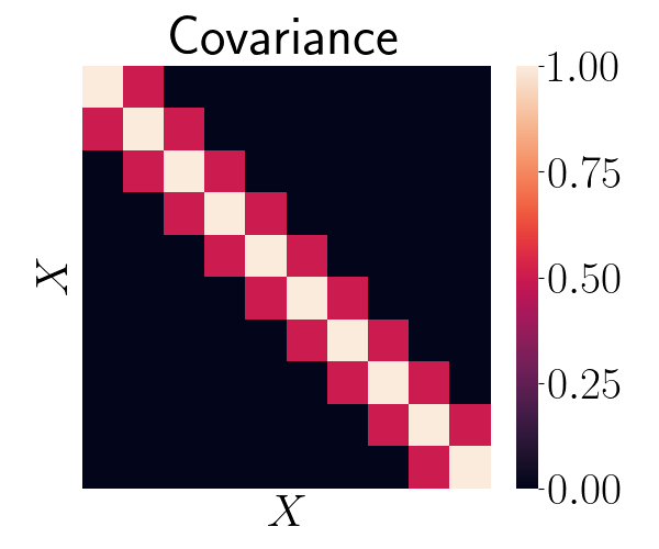
To draw a sequence, we can sample from a multivariate Gaussian with zero mean and the above covariance. In Python, we can do this as follows:
N = 10

## Temporary sequence for filling out cov matrix
correlation_seq = np.concatenate([
  np.linspace(0.1, 1, N),
  np.linspace(0.9, 0.1, N-1)
])

## Fill out cov matrix
cov_mat = np.zeros((N, N))
for ii in range(N):
  start_idx = len(correlation_seq) - N - ii
  end_idx = start_idx + N
  cov_mat[ii, :] = correlation_seq[start_idx:end_idx]

## Draw a sequence
sequence = mvn.rvs(mean=np.zeros(N), cov=cov_mat)
Suppose we’re interested in estimating the mean of $X$. To do this, we could draw a sequence as above, and compute the empirical average. However, let’s examine the variance of this estimator. To do this empirically, let’s draw $10,000$ sequences as shown above, and compute the mean for each sequence. For comparison, let’s also draw $10,000$ sequences of length $10$ where each sequence has completely uncorrelated elements (i.e., the covariance matrix is the identity). Below, we plot a histogram of the empirical averages for each of these approaches.
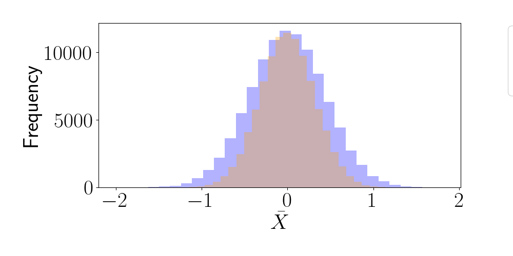
We can see that the estimator based on the correlated sequences has a higher variance than the estimator based on independent samples. In fact, our theory above predicts that the estimator based on the correlated sequences will have variance $1 / N_{\text{eff}}$, and the variance based on independent samples will have variance $1 / N$ (based on the classical CLT). Let’s compute $N_{\text{eff}}$ and validate this theory.
In this toy example, we know the ground truth autocorrelations, so we can compute the true effective sample size as well. For the correlated sequences, this is given by
\[N_{\text{eff}} = \frac{N}{1 + 2 \cdot 0.5} = \frac{10}{2} = 5.\]However, in real world situations, we wouldn’t know these quantities, but we can estimate them from the data. Here, let’s do that by computing the empirical Pearson correlation for each time lag using our sampled sequences. We find that the estimated sample size is very close to $5$.
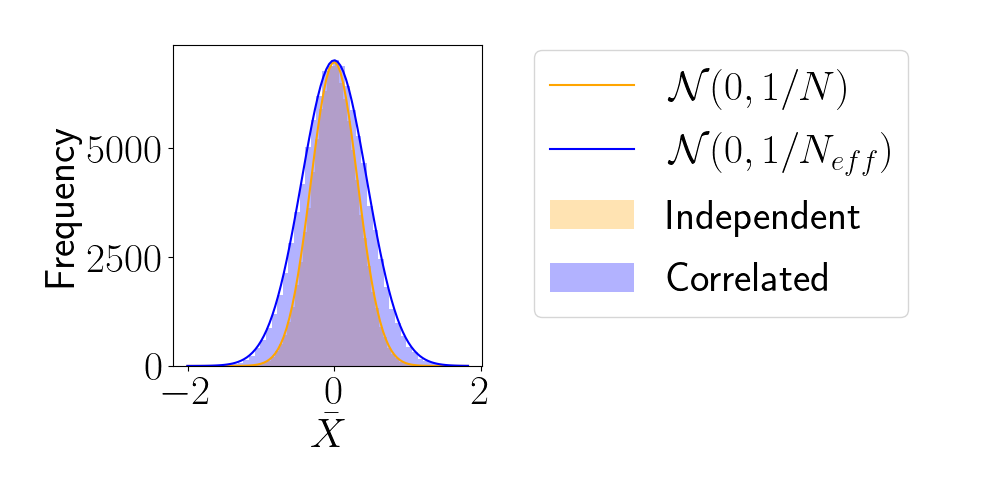
To visualize these limiting distributions, below we overlay Gaussian densities whose variances are determined by the effective sample size estimated from the data. We can see that the observed distributions match the predictions from the theory quite closely.
References
- Geyer, Charles J. “Introduction to markov chain monte carlo.” Handbook of markov chain monte carlo 20116022 (2011): 45.
- Stan handbook post on effective sample size.