Andy Jones
Dirichlet Processes
layout: post title: “Dirichlet Processes: the basics” author: “Andy Jones” categories: journal blurb: “The Dirichlet process (DP) is one of the most common – and one of the most simple – prior distributions used in Bayesian nonparametric models. In this post, we’ll review a couple different interpretations of DPs.” img: “” tags: [] —
The Dirichlet process (DP) is one of the most common – and one of the most simple – prior distributions used in Bayesian nonparametric models. In this post, we’ll review a couple different interpretations of DPs.
Dirichlet process
The Dirichlet process is a stochastic process wherein any arbitrary partition of the probability space has a Dirichlet distribution. One can think of it as a probability distribution that forms a prior for other probability distributions. In other words, a sample from a DP, $F \sim DP$, will be a probability distribution. For this reason, DPs can be used as a prior when estimating a CDF.
A DP, denoted $DP(\alpha, F_0)$ has two parameters: $F_0$ is a prior guess at the distribution in question, and $\alpha$ is a dispersion parameter that dictates how closely samples follow $F_0$.
To sample from a DP, it’s common to use a “stick-breaking” process. We present the generative process here, and explain the intuition below.
Stick-breaking process for sampling $F \sim DP(\alpha, F_0)$:
- Draw $s_1, \dots, s_\infty$ from $F_0$.
- Draw $V_1, \dots, V_\infty$ from $\text{Beta}(1, \alpha)$.
- Let $w_1 = V_1$ and $w_j = V_j \prod\limits_{i = 1}^{j - 1} (1 - V_i)$ for $j = 2, \dots \infty$.
- Let $F$ be the discrete distribution that puts mass $w_j$ at $s_j$, that is, $F = \sum\limits_{j = 1}^\infty w_j \delta_{s_j}$ where $\delta_{s_j}$ is a point mass at $s_j$.
The intuition is as follows: Imagine a stick with length $1$. Then, iteratively, we break the stick. On iteration $1$, we sample a value $V_1 \in [0, 1]$ from a Beta distribution, and break the stick at $V_1$. Now our stick has length $1 - V_1$. On iteration $2$, we sample another value $V_2 \in [0, 1]$, and break off $V_2$ fraction of the stick, leaving us with a stick of size $V_2(1 - V_1)$. We continue this process, letting the stick get smaller and smaller. The size of the stick at each iteration determines the weight placed on each point in the distribution.
Notice that the DP places more weight on samples that are early in the list of samples, and also places more weight on samples that are favored by the particular Beta distribution.
In practice, because we can’t draw infinite samples from $F_0$ in step 1, to demonstrate sampling from a DP, we truncate this to drawing $k$ samples.
We show how to perform this process in Python below, setting $F_0 = \mathcal{N}(0, 1)$ and $\alpha = 10$:
import numpy as np
from scipy.stats import beta
from scipy.stats import norm

k = 100
alpha = 10

# F_0
s = np.random.normal(0, 1, size=k)
# Beta for drawing V's
v = np.random.beta(1, alpha, size=k)

ws = [v[0]]
for ii in range(1, k):
    ws.append(v[ii] * np.prod(1 - v[:ii]))
ws = np.array(ws)
Looking at the resulting draws, we can see that it starts to resemble $F_0$, but as a discrete distribution. Here we plot the draws and their CDF.

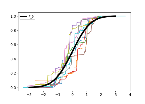
Drawing multiple samples we can start to get a sense for how much variability this prior (and our current hyperparameter settings) are allowing:
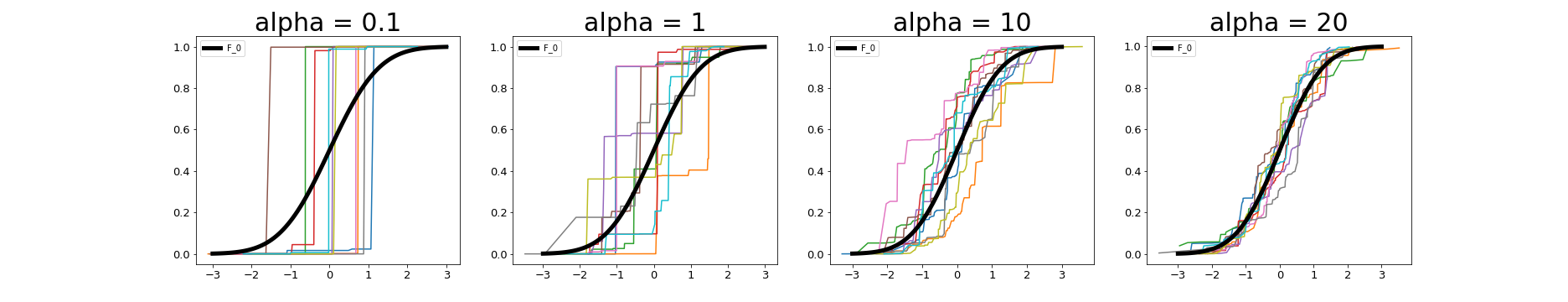
Finally, we can test how different values for $\alpha$ affect the variability of our DP draws:
References
- Prof. Larry Wasserman’s notes on Bayesian nonparametric models.
- Wikipedia page on DPs