Andy Jones
Biology of Genomes themes: A text analysis of abstracts
\(\DeclareMathOperator*{\argmin}{arg\,min}\) \(\DeclareMathOperator*{\argmax}{arg\,max}\)
I attended the 2022 Biology of Genomes meeting at Cold Spring Harbor Laboratory (CSHL) last week and was overwhelmed by the breadth of incredible science presented. While each individual talk and poster described a specific research project, I came away from the conference wanting to understand where the genomics research community was headed in aggregate. I wanted to identify a handful of research themes that could summarize the zeitgeist of the conference (and of the genomics community more generally).
In this post, I attempt to identify these themes in a data-driven manner by performing a series of simple text analyses using the titles of accepted talks and posters. These titles are only available as far back as 2016, so this analysis just includes the seven meetings from 2016 to 2022.
Scraping the talk and poster titles
Obtaining the titles for all accepted talks and posters was relatively straightforward, as they’re posted neatly in a table at the same base URL each year (with only the year number changing). Below is the simple Python script I used to grab these titles. I used the read_html function from pandas to read the HTML directly into a DataFrame.
import numpy as np
import pandas as pd

base_url = "https://meetings.cshl.edu/abstracts.aspx?meet=genome&year="

# 2016-2022 meetings
years = np.arange(16, 23)
for year in years:

  # Read table
  table = pd.read_html(base_url + str(year))

  # Get column containing titles
  assert table[0].iloc[:, 1].values[0] == "Abstract Title"

  # Save to CSV
  table[0].to_csv("./data/abstract_table_{}.csv".format(str(year)))
Tokenizing and cleaning the data
Now that I had the title of all talks and posters from each year, I used the NLTK package to split the text strings into individual tokens. I performed a couple standard processing steps, like removing punctuation, removing stop words (common words like “and” and “the”), and “lemmatizing” each word to remove plurals (e.g., “genomes” becomes “genome”) and conjugation (e.g., “ran” becomes “run”). Below is the script to perform these steps.
from nltk.corpus import stopwords
from nltk.tokenize import RegexpTokenizer, word_tokenize
from collections import Counter
import nltk
import numpy as np
import pandas as pd
import matplotlib.pyplot as plt
import seaborn as sns
from nltk.stem import WordNetLemmatizer

en_stopws = stopwords.words('english')
tokenizer = RegexpTokenizer(r'\w+')
wnl = WordNetLemmatizer()

## Read just titles
years = np.arange(16, 23)
df_list = []
for year in years:
    curr_table = pd.read_csv("./data/abstract_table_{}.csv".format(str(year)), index_col=0)
    titles = curr_table.iloc[:, 1].values[1:]
    titles_str = " ".join(titles)

    # Tokenize
    tokens = tokenizer.tokenize(titles_str)

    # Lemmatize, remove stop words, and convert to lower case
    tokens = [wnl.lemmatize(token.lower()) for token in tokens if token.lower() not in en_stopws]

    # Compute frequency of each token
    fdist = nltk.FreqDist(tokens)

    # Normalize by total counts
    total = fdist.N()
    fdist_percentages = {}
    for word in fdist.keys():
        fdist_percentages[word] = fdist[word] / total

    # Make data frame
    curr_df = pd.DataFrame.from_dict(fdist_percentages, orient='index')
    curr_df.columns = ["20" + str(year)]
    df_list.append(curr_df)

# Merge all years' dataframes
merged_df = pd.merge(df_list[0], df_list[1], left_index=True, right_index=True, how="outer")
for ii in range(2, len(df_list)):
    merged_df = pd.merge(merged_df, df_list[ii], left_index=True, right_index=True, how="outer")

# Replace missing data with 0's
merged_df = merged_df.fillna(0)
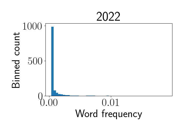
After these processing steps, we now have word-specific frequencies (percentage of each word within each year). Unsurprisingly, the distribution of word frequency follows a long-tailed distribution with most words showing very low occurrence, as we see in the histogram below for 2022 abstracts.
Identifying themes with rising popularity
As a first-pass analysis, I fit a linear model to each word’s frequency over time. Let $\mathbf{x} = (2016, \cdots, 2022)^\top$ denote the vector of years, and let $\mathbf{y}_i \in [0, 1]^7$ denote the vector of word frequencies in each year for word $i$. As further preprocessing, I performed a log transformation, i.e., transformed the data as $\log(y + 1)$ element-wise, and subtracted the mean of $\mathbf{y}_i$ to avoid the need for an intercept term. (Genomics-minded readers may notice the parallel with the typical RNA-seq or single-cell RNA-seq analysis pipeline 🤓.) To fit a linear model, I then computed the slope for each word,
\begin{equation} \widehat{\beta}_i = \frac{\mathbf{x}^\top \mathbf{y}_i}{\mathbf{x}^\top \mathbf{x}}, \label{eq:beta} \tag{1} \end{equation}
where $\widehat{\beta}_i$ is intended to capture the linear trend in popularity of word $i$ from 2016 to 2022. Let’s now look at the word frequencies over time for the 10 words with the highest $\widehat{\beta}$. The plot below shows those 10 words.
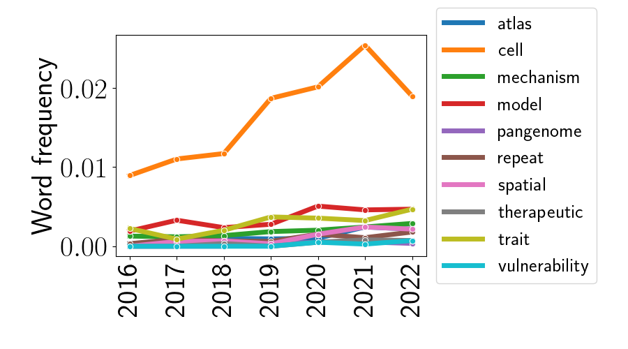
The most striking part of this plot is clearly the trend for the word “cell”. Its frequency remains much higher than all other words across all years, and its frequency seems to be rising over time (with a possible exception in 2022, although this could be just a noisy fluctuation). That the word “cell” is an outlier at a conference called “Biology of Genomes” is unsurprising, and it’s even more unsurprising given the rise of “single-cell” technologies. We’ll see this again later in this post.
To look at other trends, let’s re-plot these trends without the word “cell”.
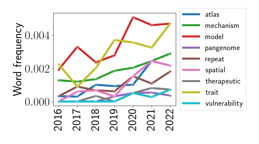
We can now notice some other interesting trends since 2016. First, the word “atlas” seems to be becoming more prevalent over time. This is perhaps due to the rise of single-cell sequencing technologies, and the subsequent rush to build “atlases” from these data that catalog cell types across tissue types and organisms. Second, the word “spatial” is also on the rise – this is also unsurprising given the rise of spatially-resolved genomics technologies in the last seven years. Third, it’s less clear why the word “model” is rising in popularity. Looking at the abstract titles that contain the word “model,” it appears to be used for a variety of different meanings. The two most popular contexts are to describe “model organisms” and “statistical or predictive models”. Perhaps it’s just the linguistic versatility of the word “model” that’s leading to its popularity. Fourth, it’s interesting that the word “mechanism” is becoming more popular – perhaps this is signaling a shift toward a lower-level understanding of the mechanistic workings of the genome.
Bigrams
Moving beyond single words, we can also look at the frequency of adjacent pairs of words (commonly called “bigrams”). I performed the same linear model analysis as above, but this time used the counts and frequencies of bigrams instead of unigrams. Below is the analogous plot as above, but for bigrams.
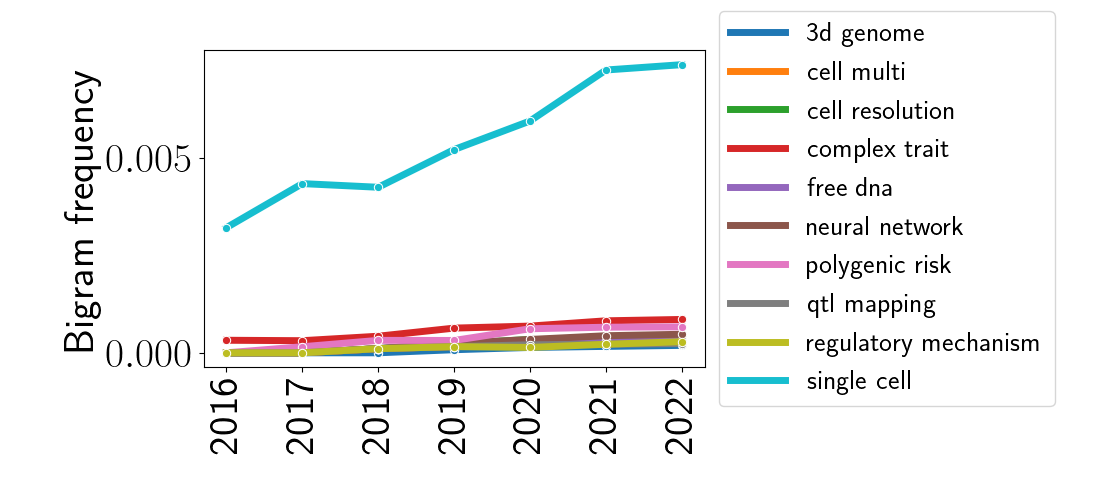
Again, the most striking feature of this plot is the bigram “single cell,” and again, this is unsurprising given the rise of technologies with single-cell resolution. To look at other bigrams, let’s remove the bigram “single cell” and re-plot these data.
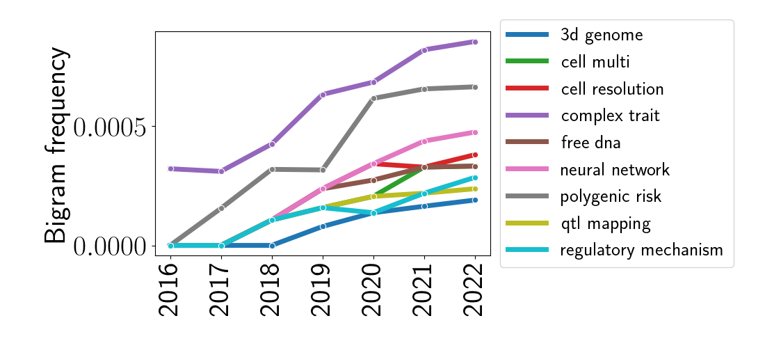
We can notice some interesting trends here. In the top-most line, we see the rise of the phrase “complex trait,” which typically refers to a phenotypic trait that cannot be explained by a single gene. These traits have received more and more attention in the QTL and GWAS analysis communities where combinations of genes and genetic loci are modeled to be associated with traits. Relatedly, we can also see a rise in the usage of “QTL mapping” and the phrase “polygenic risk,” which refers to a multi-gene or multi-locus risk factor for disease. These are often quantified in the form of “polygenic risk scores.” Finally, the popularity of neural networks appears to have grown for analyzing genomic data – this parallels a similar trend in many applied statistical and machine learning settings.
Trigrams
Extending out this analysis one more step — to trigrams — reveals a couple more interesting patterns. Again, I plotted the top ten trigrams with increasing popularity below.
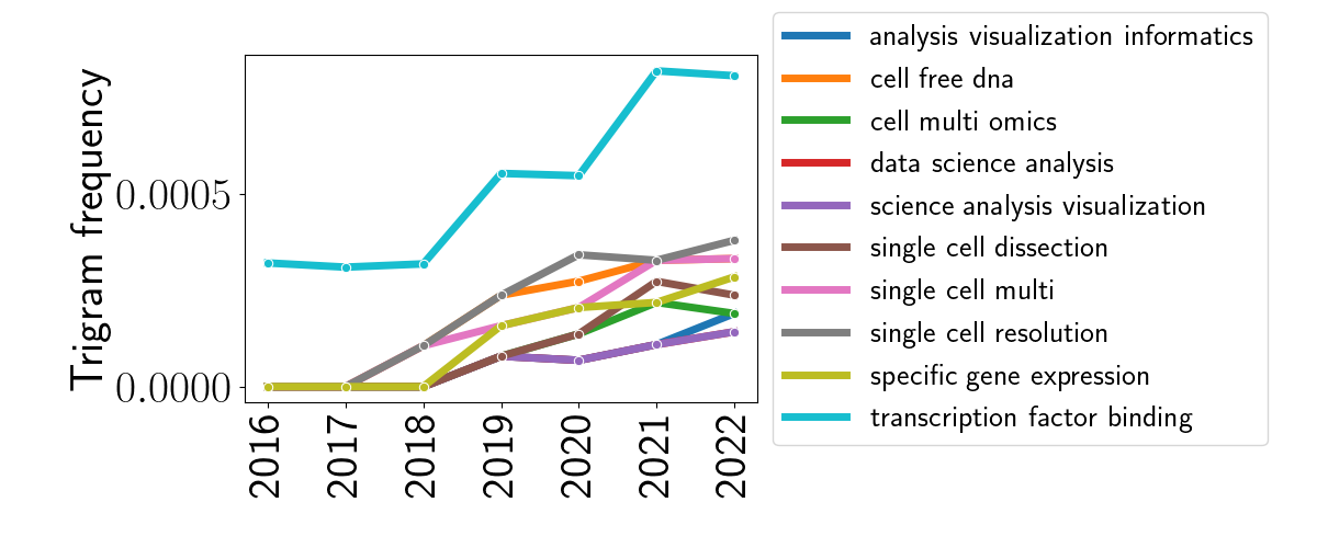
The most obvious trend here is the spike in the phrase “transcription factor binding.” This is likely due to the increase in use of epigenetic and methylation studies. Similarly, it appears that cell-free DNA — DNA that exists in the blood and isn’t encapsulated — has become more popular over the last seven years.
Identifying themes with waning popularity
While the above analysis looked at the rising trends in genomic research, we can also look at which trends are falling in popularity. Below, I plotted the 10 words with the lowest values of $\widehat{\beta}_i$ in Equation \ref{eq:beta}.
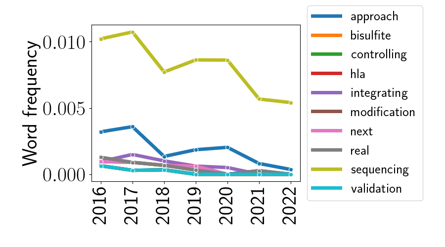
To me, it’s less clear how to interpret these downward trends compared to the upward trends we just analyzed. At the top of the plot, we see the decline of the word “sequencing.” It would be quite surprising if sequencing were actually going out of style, as most studies seem to include some amount of sequencing data or sequence analysis. However, perhaps this trend is due to the sequencing process becoming democratized and less interesting in itself. It could be that less research is focused on optimizing the sequencing process itself, and more research is focused on the sequencing data that is now easily obtained. This could explain why “sequencing” appears less frequently in abstract titles, although the word likely appears throughout the body of talks and posters. Similarly, I’m doubtful that there’s any practical significance to the word “approach” showing up here. If anything, this is maybe only indicative of a shift in general writing style.
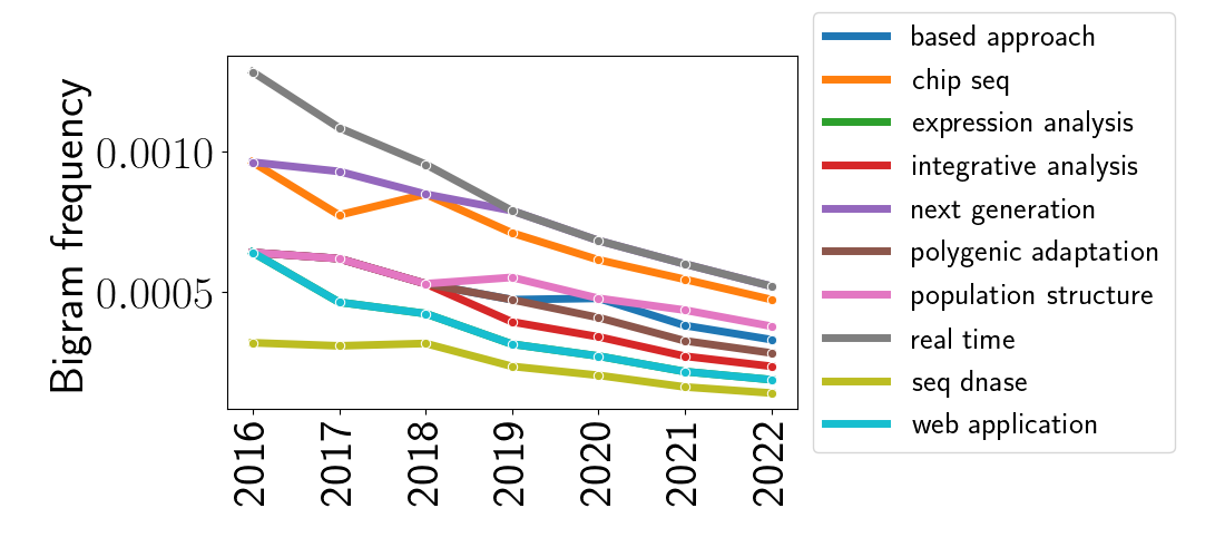
Naturally, I also extended this analysis to bigrams, as shown below.
Conclusions
The crude text analysis I presented here revealed several trends in genomic research that mirror many of the themes I noticed in last week’s 2022 meeting. If these trends continue, we should expect to see increasing research involving atlases, spatially-resolved data, complex traits, and transcription factor binding.
There are lots of things omitted from this analysis. A more rigorous way to analyze these data would be to properly model the word frequencies with a Dirichlet-multinomial-like model. Also, modeling nonlinear trends could be of interest to identify more complex patterns. For example, I suspect that words like “COVID” showed no occurrence from 2016 to 2019, likely peaked in 2020 and 2021, and fell in usage in 2022. Finally, obtaining more data from previous years would be desirable to detect longer-term shifts in the community.
Acknowledgements
Thank you to the organizers of BoG 2022 for forming an excellent conference, and thank you to all CSHL faculty and staff for hosting the meeting.